Most of the examples in this section assume that you are using an Analytics scope called Commerce.
Refer to Appendix 4: Example Data to install this example data.
You can use the USE statement to set the default scope for the statement immediately following.
USE Commerce;
Alternatively, use the query context drop-down list at the top right of the Query Editor to select Commerce as
the default scope for the following examples.

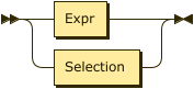
A query can be an expression, or it can be constructed from blocks of code called query blocks. A query block may contain several clauses, including SELECT, FROM, LET, WHERE, GROUP BY, and HAVING.
StreamGenerator
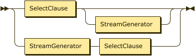
Note that, unlike SQL, SQL++ allows the SELECT clause to appear either at the beginning or at the end of a query block. For some queries, placing the SELECT clause at the end may make a query block easier to understand, because the SELECT clause refers to variables defined in the other clauses.
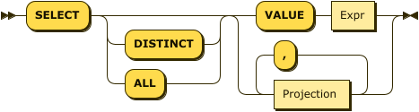
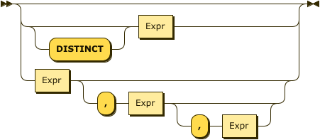
SELECT Clause
SelectClause
Projection
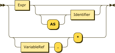
Synonyms for VALUE: ELEMENT, RAW
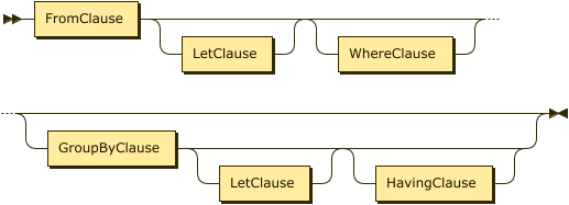
In a query block, the FROM, WHERE, GROUP BY, and HAVING clauses (if present) are collectively called the Stream Generator. All these clauses, taken together, generate a stream of tuples of bound variables. The SELECT clause then uses these bound variables to generate the output of the query block.
For example, the clause FROM customers AS c scans over the customers collection, binding the variable c to each customer object in turn, producing a stream of bindings.
Here’s a slightly more complex example of a stream generator:
FROM customers AS c, orders AS o
WHERE c.custid = o.custid
In this example, the FROM clause scans over the customers and orders collections, producing a stream of variable pairs (c, o) in which c is bound to a customer object and o is bound to an order object. The WHERE clause then retains only those pairs in which the custid values of the two objects match.
The output of the query block is a collection containing one output item for each tuple produced by the stream generator. If the stream generator produces no tuples, the output of the query block is an empty collection. Depending on the SELECT clause, each output item may be an object or some other kind of value.
In addition to using the variables bound by previous clauses, the SELECT clause may create and bind some additional variables. For example, the clause SELECT salary + bonus AS pay creates the variable pay and binds it to the value of salary + bonus. This variable may then be used in a later ORDER BY clause.
In SQL++, the SELECT clause may appear either at the beginning or at the end of a query block. Since the SELECT clause depends on variables that are bound in the other clauses, the examples in this section place SELECT at the end of the query blocks.
SELECT VALUE
The SELECT VALUE clause returns an array or multiset that contains the results of evaluating the VALUE expression, with one evaluation being performed per "binding tuple" (i.e., per FROM clause item) satisfying the statement’s selection criteria.
If there is no FROM clause, the expression after VALUE is evaluated once with no binding tuples
(except those inherited from an outer environment).
Example
(Q3.1)
SELECT VALUE 1;
Result:
[
   1
]
Example
(Q3.2) The following query returns the names of all customers whose rating is above 650.
FROM customers AS c
WHERE c.rating > 650
SELECT VALUE name;
Result:
[
    "T. Cody",
    "M. Sinclair",
    "T. Henry"
]
SQL-style SELECT
Traditional SQL-style SELECT syntax is also supported in SQL++, however the result of a query is not guaranteed to preserve the order of expressions in the SELECT clause.
Example
(Q3.3) The following query returns the names and customers ids of any customers whose rating is 750.
FROM customers AS c
WHERE c.rating = 750
SELECT c.name AS customer_name, c.custid AS customer_id;
Result:
[
    {
        "customer_id": "C13",
        "customer_name": "T. Cody"
    },
    {
        "customer_id": "C37",
        "customer_name": "T. Henry"
    }
]
SELECT *
As in SQL, the phrase SELECT * suggests, "select everything."
For each binding tuple in the stream, SELECT * produces an output object. For each variable in the binding tuple, the output object contains a field: the name of the field is the name of the variable, and the value of the field is the value of the variable. Essentially, SELECT * means, "return all the bound variables, with their names and values."
The effect of SELECT * can be illustrated by an example based on two small collections named ages and eyes. The contents of the two collections are as follows:
ages:
[
    { "name": "Bill", "age": 21 },
    { "name": "Sue", "age": 32 }
]
eyes:
[
    { "name": "Bill", "eyecolor": "brown" },
    { "name": "Sue", "eyecolor": "blue" }
]
The following example applies SELECT * to a single collection.
Example
(Q3.4a) Return all the information in the ages collection.
FROM ages AS a
SELECT * ;
Result:
[
    { "a": { "name": "Bill", "age": 21 },
    },
    { "a": { "name": "Sue", "age": 32}
    }
]
Note that the variable-name a appears in the query result. If the FROM clause had been simply FROM ages (omitting AS a), the variable-name in the query result would have been ages.
The next example applies SELECT * to a join of two collections.
Example
(Q3.4b) Return all the information in a join of ages and eyes on matching name fields.
FROM ages AS a, eyes AS e
WHERE a.name = e.name
SELECT * ;
Result:
[
    { "a": { "name": "Bill", "age": 21 },
      "e": { "name": "Bill", "eyecolor": "Brown" }
    },
    { "a": { "name": "Sue", "age": 32 },
      "e": { "name": "Sue", "eyecolor": "Blue" }
    }
]
Note that the result of SELECT * in SQL++ is more complex than the result of SELECT * in SQL.
SELECT variable.*
SQL++ has an alternative version of SELECT * in which the star is preceded by a variable.
Whereas the version without a named variable means, "return all the bound variables, with their names and values," SELECT variable .* means "return only the named variable, and return only its value, not its name."
The following example can be compared with (Q3.4a) to see the difference between the two versions of SELECT *:
Example
(Q3.4c) Return all information in the ages collection.
FROM ages AS a
SELECT a.*
Result:
[
    { "name": "Bill", "age": 21 },
    { "name": "Sue", "age": 32 }
]
Note that, for queries over a single collection, SELECT variable .* returns a simpler result and therefore may be preferable to SELECT *.
In fact, SELECT variable .*, like SELECT * in SQL, is equivalent to a SELECT clause that enumerates all the fields of the collection, as in (Q3.4d):
Example
(Q3.4d) Return all the information in the ages collection.
FROM ages AS a
SELECT a.name, a.age
(same result as (Q3.4c))
SELECT variable .* has an additional application. It can be used to return all the fields of a nested object. To illustrate this use, we will use the customers dataset in the example database — see Appendix 4.
Example
(Q3.4e) In the customers dataset, return all the fields of the address objects that have zipcode "02340".
FROM customers AS c
WHERE c.address.zipcode = "02340"
SELECT address.*  ;
Result:
[
    {
        "street": "690 River St.",
        "city": "Hanover, MA",
        "zipcode": "02340"
    }
]
SELECT DISTINCT
The DISTINCT keyword is used to eliminate duplicate items from the results of a query block.
Example
(Q3.5a) Returns all of the different cities in the customers dataset.
FROM customers AS c
SELECT DISTINCT c.address.city;
Result:
[
    {
        "city": "Boston, MA"
    },
    {
        "city": "Hanover, MA"
    },
    {
        "city": "St. Louis, MO"
    },
    {
        "city": "Rome, Italy"
    }
]
SELECT EXCLUDE
The EXCLUDE keyword is used to remove one or more fields that would otherwise be returned from the SELECT clause.
Conceptually, the scope of the EXCLUDE clause is the output of the SELECT clause itself.
In a Stream Generator with both DISTINCT and EXCLUDE clauses, the DISTINCT clause is applied after the EXCLUDE clause.
Example
(Q3.5b) For the customer with custid = C13, return their information excluding the zipcode field inside the address object and the top-level name field.
FROM customers AS c
WHERE c.custid = "C13"
SELECT c.* EXCLUDE address.zipcode, name;
Result:
[
    {
        "custid": "C13",
        "address": {
            "street": "201 Main St.",
            "city": "St. Louis, MO"
        },
        "rating": 750
    }
]
Unnamed Projections
Similar to standard SQL, the query language supports unnamed projections (a.k.a, unnamed SELECT clause items), for which names are generated rather than user-provided.
Name generation has three cases:
-
If a projection expression is a variable reference expression, its generated name is the name of the variable.
-
If a projection expression is a field access expression, its generated name is the last identifier in the expression.
-
For all other cases, the query processor will generate a unique name.
Example
(Q3.6) Returns the last digit and the order date of all orders for the customer whose ID is "C41".
FROM orders AS o
WHERE o.custid = "C41"
SELECT o.orderno % 1000,  o.order_date;
Result:
[
    {
        "$1": 1,
        "order_date": "2020-04-29"
    },
    {
        "$1": 6,
        "order_date": "2020-09-02"
    }
]
In the result, $1 is the generated name for o.orderno % 1000, while order_date is the generated name for o.order_date. It is good practice, however, to not rely on the randomly generated names which can be confusing and irrelevant. Instead, practice good naming conventions by providing a meaningful and concise name which properly describes the selected item.
Abbreviated Field Access Expressions
As in standard SQL, field access expressions can be abbreviated when there is no ambiguity. In the next example, the variable o is the only possible variable reference for fields orderno and order_date and thus could be omitted in the query. This practice is not recommended, however, as queries may have fields (such as custid) which can be present in multiple datasets. More information on abbreviated field access can be found in the appendix section on Variable Resolution.
Example
(Q3.7) Same as Q3.6, omitting the variable reference for the order number and date and providing custom names for SELECT clause items.
FROM orders AS o
WHERE o.custid = "C41"
SELECT orderno % 1000 AS last_digit, order_date;
Result:
[
    {
        "last_digit": 1,
        "order_date": "2020-04-29"
    },
    {
        "last_digit": 6,
        "order_date": "2020-09-02"
    }
]
FROM Clause
FromClause
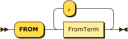
FromTerm
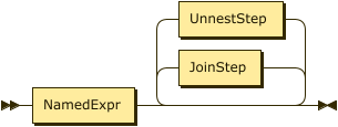
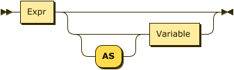
NamedExpr
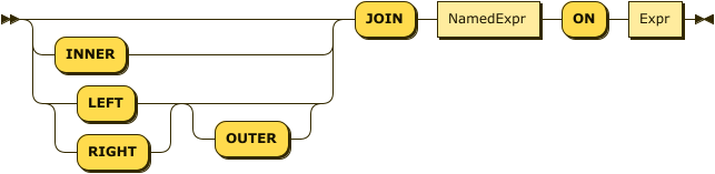
JoinStep
UnnestStep
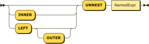
Synonyms for UNNEST: CORRELATE, FLATTEN
The purpose of a FROM clause is to iterate over a collection, binding a variable to each item in turn. Here’s a query that iterates over the customers dataset, choosing certain customers and returning some of their attributes.
Example
(Q3.8) List the customer ids and names of the customers in zipcode 63101, in order by their customer IDs.
FROM customers
WHERE address.zipcode = "63101"
SELECT custid AS customer_id, name
ORDER BY customer_id;
Result:
[
    {
        "customer_id": "C13",
        "name": "T. Cody"
    },
    {
        "customer_id": "C31",
        "name": "B. Pruitt"
    },
    {
        "customer_id": "C41",
        "name": "R. Dodge"
    }
]
Let’s take a closer look at what this FROM clause is doing. A FROM clause always produces a stream of bindings, in which an iteration variable is bound in turn to each item in a collection. In Q3.8, since no explicit iteration variable is provided, the FROM clause defines an implicit variable named customers, the same name as the dataset that is being iterated over. The implicit iteration variable serves as the object-name for all field-names in the query block that do not have explicit object-names. Thus, address.zipcode really means customers.address.zipcode, custid really means customers.custid, and name really means customers.name.
You may also provide an explicit iteration variable, as in this version of the same query:
Example
(Q3.9) Alternative version of Q3.8 (same result).
FROM customers AS c
WHERE c.address.zipcode = "63101"
SELECT c.custid AS customer_id, c.name
ORDER BY customer_id;
In Q3.9, the variable c is bound to each customer object in turn as the query iterates over the customers dataset. An explicit iteration variable can be used to identify the fields of the referenced object, as in c.name in the SELECT clause of Q3.9. When referencing a field of an object, the iteration variable can be omitted when there is no ambiguity. For example, c.name could be replaced by name in the SELECT clause of Q3.9. That’s why field-names like name and custid could stand by themselves in the Q3.8 version of this query.
In the examples above, the FROM clause iterates over the objects in a dataset. But in general, a FROM clause can iterate over any collection. For example, the objects in the orders dataset each contain a field called items, which is an array of nested objects. In some cases, you will write a FROM clause that iterates over a nested array like items.
The stream of objects (more accurately, variable bindings) that is produced by the FROM clause does not have any particular order. The system will choose the most efficient order for the iteration. If you want your query result to have a specific order, you must use an ORDER BY clause.
It’s good practice to specify an explicit iteration variable for each collection in the FROM clause, and to use these variables to qualify the field-names in other clauses. Here are some reasons for this convention:
-
It’s nice to have different names for the collection as a whole and an object in the collection. For example, in the clause
FROM customers AS c, the namecustomersrepresents the dataset and the namecrepresents one object in the dataset. -
In some cases, iteration variables are required. For example, when joining a dataset to itself, distinct iteration variables are required to distinguish the left side of the join from the right side.
-
In a subquery it’s sometimes necessary to refer to an object in an outer query block (this is called a correlated subquery). To avoid confusion in correlated subqueries, it’s best to use explicit variables.
Joins
A FROM clause gets more interesting when there is more than one collection involved. The following query iterates over two collections: customers and orders. The FROM clause produces a stream of binding tuples, each containing two variables, c and o. In each binding tuple, c is bound to an object from customers, and o is bound to an object from orders. Conceptually, at this point, the binding tuple stream contains all possible pairs of a customer and an order (this is called the Cartesian product of customers and orders). Of course, we are interested only in pairs where the custid fields match, and that condition is expressed in the WHERE clause, along with the restriction that the order number must be 1001.
Example
(Q3.10) Create a packing list for order number 1001, showing the customer name and address and all the items in the order.
FROM customers AS c, orders AS o
WHERE c.custid = o.custid
AND o.orderno = 1001
SELECT o.orderno,
    c.name AS customer_name,
    c.address,
    o.items AS items_ordered;
Result:
[
    {
        "orderno": 1001,
        "customer_name": "R. Dodge",
        "address": {
            "street": "150 Market St.",
            "city": "St. Louis, MO",
            "zipcode": "63101"
        },
        "items_ordered": [
            {
                "itemno": 347,
                "qty": 5,
                "price": 19.99
            },
            {
                "itemno": 193,
                "qty": 2,
                "price": 28.89
            }
        ]
    }
]
Q3.10 is called a join query because it joins the customers collection and the orders collection, using the join condition c.custid = o.custid. In SQL++, as in SQL, you can express this query more explicitly by a JOIN clause that includes the join condition, as follows:
Example
(Q3.11) Alternative statement of Q3.10 (same result).
FROM customers AS c JOIN orders AS o
    ON c.custid = o.custid
WHERE o.orderno = 1001
SELECT o.orderno,
    c.name AS customer_name,
    c.address,
    o.items AS items_ordered;
Whether you express the join condition in a JOIN clause or in a WHERE clause is a matter of taste; the result is the same. This manual will generally use a comma-separated list of collection-names in the FROM clause, leaving the join condition to be expressed elsewhere. As we’ll soon see, in some query blocks the join condition can be omitted entirely.
There is, however, one case in which an explicit JOIN clause is necessary. That is when you need to join collection A to collection B, and you want to make sure that every item in collection A is present in the query result, even if it doesn’t match any item in collection B. This kind of query is called a left outer join, and it is illustrated by the following example.
Example
(Q3.12) List the customer ID and name, together with the order numbers and dates of their orders (if any) of customers T. Cody and M. Sinclair.
FROM customers AS c LEFT OUTER JOIN orders AS o ON c.custid = o.custid
WHERE c.name = "T. Cody"
   OR c.name = "M. Sinclair"
SELECT c.custid, c.name, o.orderno, o.order_date
ORDER BY c.custid, o.order_date;
Result:
[
    {
        "custid": "C13",
        "orderno": 1002,
        "name": "T. Cody",
        "order_date": "2020-05-01"
    },
    {
        "custid": "C13",
        "orderno": 1007,
        "name": "T. Cody",
        "order_date": "2020-09-13"
    },
    {
        "custid": "C13",
        "orderno": 1008,
        "name": "T. Cody",
        "order_date": "2020-10-13"
    },
    {
        "custid": "C13",
        "orderno": 1009,
        "name": "T. Cody",
        "order_date": "2020-10-13"
    },
    {
        "custid": "C25",
        "name": "M. Sinclair"
    }
]
As you can see from the result of this left outer join, our data includes four orders from customer T. Cody, but no orders from customer M. Sinclair. The behavior of left outer join in SQL++ is different from that of SQL. SQL would have provided M. Sinclair with an order in which all the fields were null. SQL++, on the other hand, deals with schemaless data, which permits it to simply omit the order fields from the outer join.
Now we’re ready to look at a new kind of join that was not provided (or needed) in original SQL. Consider this query:
Example
(Q3.13) For every case in which an item is ordered in a quantity greater than 100, show the order number, date, item number, and quantity.
FROM orders AS o, o.items AS i
WHERE i.qty > 100
SELECT o.orderno, o.order_date, i.itemno AS item_number,
    i.qty AS quantity
ORDER BY o.orderno, item_number;
Result:
[
    {
        "orderno": 1002,
        "order_date": "2020-05-01",
        "item_number": 680,
        "quantity": 150
    },
    {
        "orderno": 1005,
        "order_date": "2020-08-30",
        "item_number": 347,
        "quantity": 120
    },
    {
        "orderno": 1006,
        "order_date": "2020-09-02",
        "item_number": 460,
        "quantity": 120
    }
]
Q3.13 illustrates a feature called left-correlation in the FROM clause. Notice that we are joining orders, which is a dataset, to items, which is an array nested inside each order. In effect, for each order, we are unnesting the items array and joining it to the order as though it were a separate collection. For this reason, this kind of query is sometimes called an unnesting query. The keyword UNNEST may be used whenever left-correlation is used in a FROM clause, as shown in this example:
Example
(Q3.14) Alternative statement of Q3.13 (same result).
FROM orders AS o UNNEST o.items AS i
WHERE i.qty > 100
SELECT o.orderno, o.order_date, i.itemno AS item_number,
        i.qty AS quantity
ORDER BY o.orderno, item_number;
The results of Q3.13 and Q3.14 are exactly the same. UNNEST serves as a reminder that left-correlation is being used to join an object with its nested items. The join condition in Q3.14 is expressed by the left-correlation: each order o is joined to its own items, referenced as o.items. The result of the FROM clause is a stream of binding tuples, each containing two variables, o and i. The variable o is bound to an order and the variable i is bound to one item inside that order.
Like JOIN, UNNEST has a LEFT OUTER option. Q3.14 could have specified:
FROM orders AS o LEFT OUTER UNNEST o.items AS i
In this case, orders that have no nested items would appear in the query result.
LET Clause
LetClause
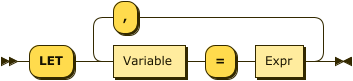
Synonyms for LET: LETTING
LET clauses can be useful when a (complex) expression is used several times within a query, allowing it to be written once to make the query more concise. The word LETTING can also be used, although this is not as common. The next query shows an example.
Example
(Q3.15) For each item in an order, the revenue is defined as the quantity times the price of that item. Find individual items for which the revenue is greater than 5000. For each of these, list the order number, item number, and revenue, in descending order by revenue.
FROM orders AS o, o.items AS i
LET revenue = i.qty * i.price
WHERE revenue > 5000
SELECT o.orderno, i.itemno, revenue
ORDER by revenue desc;
Result:
[
    {
        "orderno": 1006,
        "itemno": 460,
        "revenue": 11997.6
    },
    {
        "orderno": 1002,
        "itemno": 460,
        "revenue": 9594.05
    },
    {
        "orderno": 1006,
        "itemno": 120,
        "revenue": 5525
    }
]
The expression for computing revenue is defined once in the LET clause and then used three times in the remainder of the query. Avoiding repetition of the revenue expression makes the query shorter and less prone to errors.
WHERE Clause
WhereClause

The purpose of a WHERE clause is to operate on the stream of binding tuples generated by the FROM clause, filtering out the tuples that do not satisfy a certain condition. The condition is specified by an expression based on the variable names in the binding tuples. If the expression evaluates to true, the tuple remains in the stream; if it evaluates to anything else, including null or missing, it is filtered out. The surviving tuples are then passed along to the next clause to be processed (usually either GROUP BY or SELECT).
Often, the expression in a WHERE clause is some kind of comparison like quantity > 100. However, any kind of expression is allowed in a WHERE clause. The only thing that matters is whether the expression returns true or not.
Grouping
Grouping is especially important when manipulating hierarchies like the ones that are often found in JSON data. Often you will want to generate output data that includes both summary data and line items within the summaries. For this purpose, SQL++ supports several important extensions to the traditional grouping features of SQL. The familiar GROUP BY and HAVING clauses are still there, and they are joined by a new clause called GROUP AS. We’ll illustrate these clauses by a series of examples.
GROUP BY Clause
GroupByClause
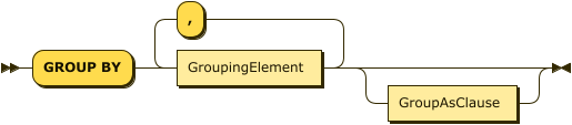
GroupingElement
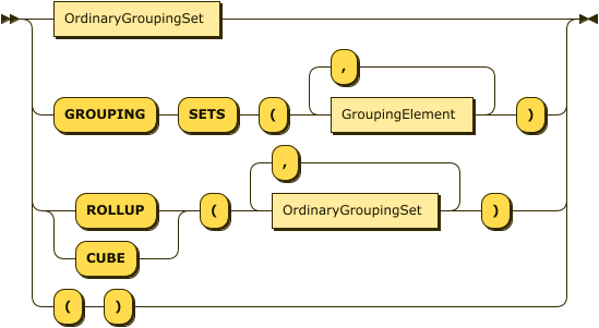
OrdinaryGroupingSet
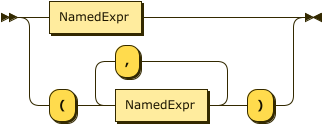
NamedExpr
We’ll begin our discussion of grouping with an example from ordinary SQL.
Example
(Q3.16) List the number of orders placed by each customer who has placed an order.
SELECT o.custid, COUNT(o.orderno) AS `order count`
FROM orders AS o
GROUP BY o.custid
ORDER BY o.custid;
Result:
[
    {
        "order count": 4,
        "custid": "C13"
    },
    {
        "order count": 1,
        "custid": "C31"
    },
    {
        "order count": 1,
        "custid": "C35"
    },
    {
        "order count": 1,
        "custid": "C37"
    },
    {
        "order count": 2,
        "custid": "C41"
    }
]
The input to a GROUP BY clause is the stream of binding tuples generated by the FROM and WHEREclauses. In this query, before grouping, the variable o is bound to each object in the orders collection in turn.
SQL++ evaluates the expression in the GROUP BY clause, called the grouping expression, once for each of the binding tuples. It then organizes the results into groups in which the grouping expression has a common value (as defined by the = operator). In this example, the grouping expression is o.custid, and each of the resulting groups is a set of orders that have the same custid. If necessary, a group is formed for orders in which custid is null, and another group is formed for orders that have no custid. This query uses the aggregating function COUNT(o.orderno), which counts how many order numbers are in each group. If we are sure that each order object has a distinct orderno, we could also simply count the order objects in each group by using COUNT(*) in place of COUNT(o.orderno).
In the GROUP BYclause, you may optionally define an alias for the grouping expression. For example, in Q3.16, you could have written GROUP BY o.custid AS cid. The alias cid could then be used in place of the grouping expression in later clauses. In cases where the grouping expression contains an operator, it is especially helpful to define an alias (for example, GROUP BY salary + bonus AS pay).
Q3.16 had a single grouping expression, o.custid. If a query has multiple grouping expressions, the combination of grouping expressions is evaluated for every binding tuple, and the stream of binding tuples is partitioned into groups that have values in common for all of the grouping expressions. We’ll see an example of such a query in Q3.18.
After grouping, the number of binding tuples is reduced: instead of a binding tuple for each of the input objects, there is a binding tuple for each group. The grouping expressions (identified by their aliases, if any) are bound to the results of their evaluations. However, all the non-grouping fields (that is, fields that were not named in the grouping expressions), are accessible only in a special way: as an argument of one of the special aggregation pseudo-functions such as: SUM, AVG, MAX, MIN, STDEV and COUNT. The clauses that come after grouping can access only properties of groups, including the grouping expressions and aggregate properties of the groups such as COUNT(o.orderno) or COUNT(*). (We’ll see an exception when we discuss the new GROUP AS clause.)
You may notice that the results of Q3.16 do not include customers who have no orders. If we want to include these customers, we need to use an outer join between the customers and orders collections. This is illustrated by the following example, which also includes the name of each customer.
Example
(Q3.17) List the number of orders placed by each customer including those customers who have placed no orders.
SELECT c.custid, c.name, COUNT(o.orderno) AS `order count`
FROM customers AS c LEFT OUTER JOIN orders AS o ON c.custid = o.custid
GROUP BY c.custid, c.name
ORDER BY c.custid;
Result:
[
    {
        "custid": "C13",
        "order count": 4,
        "name": "T. Cody"
    },
    {
        "custid": "C25",
        "order count": 0,
        "name": "M. Sinclair"
    },
    {
        "custid": "C31",
        "order count": 1,
        "name": "B. Pruitt"
    },
    {
        "custid": "C35",
        "order count": 1,
        "name": "J. Roberts"
    },
    {
        "custid": "C37",
        "order count": 1,
        "name": "T. Henry"
    },
    {
        "custid": "C41",
        "order count": 2,
        "name": "R. Dodge"
    },
    {
        "custid": "C47",
        "order count": 0,
        "name": "S. Logan"
    }
]
Notice in Q3.17 what happens when the special aggregation function COUNT is applied to a collection that does not exist, such as the orders of M. Sinclair: it returns zero. This behavior is unlike that of the other special aggregation functions SUM, AVG, MAX, and MIN, which return null if their operand does not exist. This should make you cautious about the COUNT function: If it returns zero, that may mean that the collection you are counting has zero members, or that it does not exist, or that you have misspelled the collection’s name.
Q3.17 also shows how a query block can have more than one grouping expression. In general, the GROUP BYclause produces a binding tuple for each different combination of values for the grouping expressions. In Q3.17, the c.custid field uniquely identifies a customer, so adding c.name as a grouping expression does not result in any more groups. Nevertheless, c.name must be included as a grouping expression if it is to be referenced outside (after) the GROUP BY clause. If c.name were not included in the GROUP BY clause, it would not be a group property and could not be used in the SELECT clause.
Of course, a grouping expression need not be a simple field-name. In Q3.18, orders are grouped by month, using a temporal function to extract the month component of the order dates. In cases like this, it is helpful to define an alias for the grouping expression so that it can be referenced elsewhere in the query e.g. in the SELECT clause.
Example
(Q3.18) Find the months in 2020 that had the largest numbers of orders; list the months and their numbers of orders. (Return the top three.)
FROM orders AS o
WHERE DATE_PART_STR(o.order_date, "year") = 2020
GROUP BY DATE_PART_STR(o.order_date, "month") AS month
SELECT month, COUNT(*) AS order_count
ORDER BY order_count DESC, month DESC
LIMIT 3;
Result:
[
    {
        "month": 10,
        "order_count": 2
    },
    {
        "month": 9,
        "order_count": 2
    },
    {
        "month": 8,
        "order_count": 1
    }
]
Groups are commonly formed from named collections like customers and orders. But in some queries you need to form groups from a collection that is nested inside another collection, such as items inside orders. In SQL++ you can do this by using left-correlation in the FROM clause to unnest the inner collection, joining the inner collection with the outer collection, and then performing the grouping on the join, as illustrated in Q3.19.
Q3.19 also shows how a LET clause can be used after a GROUP BY clause to define an expression that is referenced multiple times in later clauses.
Example
(Q3.19) For each order, define the total revenue of the order as the sum of quantity times price for all the items in that order. List the total revenue for all the orders placed by the customer with id "C13", in descending order by total revenue.
FROM orders as o, o.items as i
WHERE o.custid = "C13"
GROUP BY o.orderno
LET total_revenue = sum(i.qty * i.price)
SELECT o.orderno, total_revenue
ORDER BY total_revenue desc;
Result:
[
    {
        "orderno": 1002,
        "total_revenue": 10906.55
    },
    {
        "orderno": 1008,
        "total_revenue": 1999.8
    },
    {
        "orderno": 1007,
        "total_revenue": 130.45
    }
]
ROLLUP
The ROLLUP subclause is an aggregation feature that extends the functionality of the GROUP BY clause.
It returns extra super-aggregate items in the query results, giving subtotals and a grand total for the aggregate
functions in the query.
To illustrate, first consider the following query.
Example
(Q3.R1) List the number of orders, grouped by customer region and city.
SELECT customer_region AS Region,
       customer_city AS City,
       COUNT(o.orderno) AS `Order Count`
FROM customers AS c LEFT OUTER JOIN orders AS o ON c.custid = o.custid
LET address_line = SPLIT(c.address.city, ","),
    customer_city = TRIM(address_line[0]),
    customer_region = TRIM(address_line[1])
GROUP BY customer_region, customer_city
ORDER BY customer_region ASC, customer_city ASC, `Order Count` DESC;
Result:
[
  {
    "Region": "Italy",
    "City": "Rome",
    "Order Count": 0
  },
  {
    "Region": "MA",
    "City": "Boston",
    "Order Count": 2
  },
  {
    "Region": "MA",
    "City": "Hanover",
    "Order Count": 0
  },
  {
    "Region": "MO",
    "City": "St. Louis",
    "Order Count": 7
  }
]
This query uses string functions to split each customer’s address into city and region.
The query then counts the total number of orders placed by each customer, and groups the results first by customer
region, then by customer city.
The aggregate results (labeled Order Count) are only shown by city, and there are no subtotals or grand total.
We can add these using the ROLLUP subclause, as in the following example.
Example
(Q3.R2) List the number of orders by customer region and city, including subtotals and a grand total.
SELECT customer_region AS Region,
       customer_city AS City,
       COUNT(o.orderno) AS `Order Count`
FROM customers AS c LEFT OUTER JOIN orders AS o ON c.custid = o.custid
LET address_line = SPLIT(c.address.city, ","),
    customer_city = TRIM(address_line[0]),
    customer_region = TRIM(address_line[1])
GROUP BY ROLLUP(customer_region, customer_city)
ORDER BY customer_region ASC, customer_city ASC, `Order Count` DESC;
Result:
[
  {
    "Region": null,
    "City": null,
    "Order Count": 9
  },
  {
    "Region": "Italy",
    "City": null,
    "Order Count": 0
  },
  {
    "Region": "Italy",
    "City": "Rome",
    "Order Count": 0
  },
  {
    "Region": "MA",
    "City": null,
    "Order Count": 2
  },
  {
    "Region": "MA",
    "City": "Boston",
    "Order Count": 2
  },
  {
    "Region": "MA",
    "City": "Hanover",
    "Order Count": 0
  },
  {
    "Region": "MO",
    "City": null,
    "Order Count": 7
  },
  {
    "Region": "MO",
    "City": "St. Louis",
    "Order Count": 7
  }
]
With the addition of the ROLLUP subclause, the results now include an extra item at the start of each region,
giving the subtotal for that region.
There is also another extra item at the very start of the results, giving the grand total for all regions.
The order of the fields specified by the ROLLUP subclause determines the hierarchy of the super-aggregate items.
The customer region is specified first, followed by the customer city; so the results are aggregated by region first,
and then by city within each region.
The grand total returns null as a value for the city and the region, and the subtotals return null as the
value for the city, which may make the results hard to understand at first glance.
A workaround for this is given in the next example.
Example
(Q3.R3) List the number of orders by customer region and city, with meaningful subtotals and grand total.
SELECT IFNULL(customer_region, "All regions") AS Region,
       IFNULL(customer_city, "All cities") AS City,
       COUNT(o.orderno) AS `Order Count`
FROM customers AS c LEFT OUTER JOIN orders AS o ON c.custid = o.custid
LET address_line = SPLIT(c.address.city, ","),
    customer_city = TRIM(address_line[0]),
    customer_region = TRIM(address_line[1])
GROUP BY ROLLUP(customer_region, customer_city)
ORDER BY customer_region ASC, customer_city ASC, `Order Count` DESC;
Result:
[
  {
    "Region": "All regions",
    "City": "All cities",
    "Order Count": 9
  },
  {
    "Region": "Italy",
    "City": "All cities",
    "Order Count": 0
  },
  {
    "Region": "Italy",
    "City": "Rome",
    "Order Count": 0
  },
  {
    "Region": "MA",
    "City": "All cities",
    "Order Count": 2
  },
  {
    "Region": "MA",
    "City": "Boston",
    "Order Count": 2
  },
  {
    "Region": "MA",
    "City": "Hanover",
    "Order Count": 0
  },
  {
    "Region": "MO",
    "City": "All cities",
    "Order Count": 7
  },
  {
    "Region": "MO",
    "City": "St. Louis",
    "Order Count": 7
  }
]
This query uses the IFNULL function to populate the region and city fields with meaningful values for the
super-aggregate items.
This makes the results clearer and more readable.
CUBE
The CUBE subclause is similar to the ROLLUP subclause, in that it returns extra super-aggregate items in the query
results, giving subtotals and a grand total for the aggregate functions.
Whereas ROLLUP returns a grand total and a hierarchy of subtotals based on the specified fields,
the CUBE subclause returns a grand total and subtotals for every possible combination of the specified fields.
The following example is a modification of Q3.R3 which illustrates the CUBE subclause.
Example
(Q3.C) List the number of orders by customer region and order date, with all possible subtotals and a grand total.
SELECT IFNULL(customer_region, "All regions") AS Region,
       IFNULL(order_month, "All months") AS Month,
       COUNT(o.orderno) AS `Order Count`
FROM customers AS c INNER JOIN orders AS o ON c.custid = o.custid
LET address_line = SPLIT(c.address.city, ","),
    customer_region = TRIM(address_line[1]),
    order_month = DATE_PART_STR(o.order_date, "month")
GROUP BY CUBE(customer_region, order_month)
ORDER BY customer_region ASC, order_month ASC;
Result:
[
  {
    "Region": "All regions",
    "Order Count": 9,
    "Month": "All months"
  },
  {
    "Region": "All regions",
    "Order Count": 1,
    "Month": 4
  },
  {
    "Region": "All regions",
    "Order Count": 1,
    "Month": 5
  },
  {
    "Region": "All regions",
    "Order Count": 1,
    "Month": 6
  },
  {
    "Region": "All regions",
    "Order Count": 1,
    "Month": 7
  },
  {
    "Region": "All regions",
    "Order Count": 1,
    "Month": 8
  },
  {
    "Region": "All regions",
    "Order Count": 2,
    "Month": 9
  },
  {
    "Region": "All regions",
    "Order Count": 2,
    "Month": 10
  },
  {
    "Region": "MA",
    "Order Count": 2,
    "Month": "All months"
  },
  {
    "Region": "MA",
    "Order Count": 1,
    "Month": 7
  },
  {
    "Region": "MA",
    "Order Count": 1,
    "Month": 8
  },
  {
    "Region": "MO",
    "Order Count": 7,
    "Month": "All months"
  },
  {
    "Region": "MO",
    "Order Count": 1,
    "Month": 4
  },
  {
    "Region": "MO",
    "Order Count": 1,
    "Month": 5
  },
  {
    "Region": "MO",
    "Order Count": 1,
    "Month": 6
  },
  {
    "Region": "MO",
    "Order Count": 2,
    "Month": 9
  },
  {
    "Region": "MO",
    "Order Count": 2,
    "Month": 10
  }
]
To simplify the results, this query uses an inner join, so that customers who have not placed an order are not included in the totals. The query uses string functions to extract the region from each customer’s address, and a temporal function to extract the year from the order date.
The query uses the CUBE subclause with customer region and order month.
This means that there are four possible aggregates to calculate:
-
All regions, all months
-
All regions, each month
-
Each region, all months
-
Each region, each month
The results start with the grand total, showing the total number of orders across all regions for all months. This is followed by date subtotals, showing the number of orders across all regions for each month. Following that are the regional subtotals, showing the total number of orders for all months in each region; and the result items, giving the number of orders for each month in each region.
The query also uses the IFNULL function to populate the region and date fields with meaningful values for the
super-aggregate items.
This makes the results clearer and more readable.
HAVING Clause
HavingClause
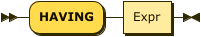
The HAVING clause is very similar to the WHERE clause, except that it comes after GROUP BY and applies a filter to groups rather than to individual objects. Here’s an example of a HAVING clause that filters orders by applying a condition to their nested arrays of items.
By adding a HAVING clause to Q3.19, we can filter the results to include only those orders whose total revenue is greater than 1000, as shown in Q3.22.
Example
(Q3.20) Modify Q3.19 to include only orders whose total revenue is greater than 5000.
FROM orders AS o, o.items as i
WHERE o.custid = "C13"
GROUP BY o.orderno
LET total_revenue = sum(i.qty * i.price)
HAVING total_revenue > 5000
SELECT o.orderno, total_revenue
ORDER BY total_revenue desc;
Result:
[
    {
        "orderno": 1002,
        "total_revenue": 10906.55
    }
]
Aggregation Pseudo-Functions
SQL provides several special functions for performing aggregations on groups including: SUM, AVG, MAX, MIN, and COUNT (some implementations provide more). These same functions are supported in SQL++. However, it’s worth spending some time on these special functions because they don’t behave like ordinary functions. They are called "pseudo-functions" here because they don’t evaluate their operands in the same way as ordinary functions. To see the difference, consider these two examples, which are syntactically similar:
SELECT LENGTH(name) FROM customers
In Example 1, LENGTH is an ordinary function. It simply evaluates its operand (name) and then returns a result computed from the operand.
SELECT AVG(rating) FROM customers
The effect of AVG in Example 2 is quite different. Rather than performing a computation on an individual rating value, AVG has a global effect: it effectively restructures the query. As a pseudo-function, AVG requires its operand to be a group; therefore, it automatically collects all the rating values from the query block and forms them into a group.
The aggregation pseudo-functions always require their operand to be a group. In some queries, the group is explicitly generated by a GROUP BY clause, as in Q3.21:
Example
(Q3.21) List the average credit rating of customers by zipcode.
FROM customers AS c
GROUP BY c.address.zipcode AS zip
SELECT zip, AVG(c.rating) AS `avg credit rating`
ORDER BY zip;
Result:
[
    {
        "avg credit rating": 625
    },
    {
        "avg credit rating": 657.5,
        "zip": "02115"
    },
    {
        "avg credit rating": 690,
        "zip": "02340"
    },
    {
        "avg credit rating": 695,
        "zip": "63101"
    }
]
Note in the result of Q3.21 that one or more customers had no zipcode. These customers were formed into a group for which the value of the grouping key is missing. When the query results were returned in JSON format, the missing key simply does not appear. Also note that the group whose key is missing appears first because missing is considered to be smaller than any other value. If some customers had had null as a zipcode, they would have been included in another group, appearing after the missing group but before the other groups.
When an aggregation pseudo-function is used without an explicit GROUP BY clause, it implicitly forms the entire query block into a single group, as in Q3.22:
Example
(Q3.22) Find the average credit rating among all customers.
FROM customers AS c
SELECT AVG(c.rating) AS `avg credit rating`;
Result:
[
    {
        "avg credit rating": 670
    }
]
The aggregation pseudo-function COUNT has a special form in which its operand is * instead of an expression.
For example, SELECT COUNT(*) FROM customers simply returns the total number of customers, whereas SELECT COUNT(rating) FROM customers returns the number of customers who have known ratings (that is, their ratings are not null or missing).
Because the aggregation pseudo-functions sometimes restructure their operands, they can be used only in query blocks where (explicit or implicit) grouping is being done. Therefore the pseudo-functions cannot operate directly on arrays or multisets. For operating directly on JSON collections, SQL++ provides a set of ordinary functions for computing aggregations. Each ordinary aggregation function (except as noted below) has two versions: one that ignores null and missing values, and one that returns null if a null or missing value is encountered anywhere in the collection. The names of the aggregation functions are as follows:
| Aggregation pseudo-function; operates on groups only | Ordinary function: Ignores NULL or MISSING values | Ordinary function: Returns NULL if NULL or MISSING are encountered |
|---|---|---|
SUM |
ARRAY_SUM |
STRICT_SUM |
AVG |
ARRAY_AVG |
STRICT_AVG |
MAX |
ARRAY_MAX |
STRICT_MAX |
MIN |
ARRAY_MIN |
STRICT_MIN |
COUNT |
ARRAY_COUNT |
STRICT_COUNT (see exception below) |
MEDIAN |
ARRAY_MEDIAN |
|
STDDEV_SAMP |
ARRAY_STDDEV_SAMP |
STRICT_STDDEV_SAMP |
STDDEV_POP |
ARRAY_STDDEV_POP |
STRICT_STDDEV_POP |
VAR_SAMP |
ARRAY_VAR_SAMP |
STRICT_VAR_SAMP |
VAR_POP |
ARRAY_VAR_POP |
STRICT_VAR_POP |
SKEWNESS |
ARRAY_SKEWNESS |
STRICT_SKEWNESS |
KURTOSIS |
ARRAY_KURTOSIS |
STRICT_KURTOSIS |
ARRAY_AGG |
Exception: the ordinary aggregation function STRICT_COUNT operates on any collection, and returns a count of its items, including null values in the count. In this respect, STRICT_COUNT is more similar to COUNT(*) than to COUNT(expression).
Note that the ordinary aggregation functions that ignore null have names beginning with "ARRAY". This naming convention has historical roots. Despite their names, the functions operate on both arrays and multisets.
Because of the special properties of the aggregation pseudo-functions, SQL (and therefore SQL++) is not a pure functional language. But every query that uses a pseudo-function can be expressed as an equivalent query that uses an ordinary function. Q3.23 is an example of how queries can be expressed without pseudo-functions. A more detailed explanation of all of the functions is also available in the section on Aggregate Functions.
Example
(Q3.23) Alternative form of Q3.22, using the ordinary function ARRAY_AVG rather than the aggregating pseudo-function AVG.
SELECT ARRAY_AVG(
    (SELECT VALUE c.rating
    FROM customers AS c) ) AS `avg credit rating`;
Result (same as Q3.22):
[
    {
        "avg credit rating": 670
    }
]
If the function STRICT_AVG had been used in Q3.23 in place of ARRAY_AVG, the average credit rating returned by the query would have been null, because at least one customer has no credit rating.
GROUP AS Clause
GroupAsClause
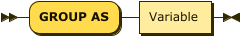
JSON is a hierarchical format, and a fully featured JSON query language needs to be able to produce hierarchies of its own, with computed data at every level of the hierarchy. The key feature of SQL++ that makes this possible is the GROUP AS clause.
A query may have a GROUP AS clause only if it has a GROUP BY clause. The GROUP BY clause "hides" the original objects in each group, exposing only the grouping expressions and special aggregation functions on the non-grouping fields. The purpose of the GROUP AS clause is to make the original objects in the group visible to subsequent clauses. Thus the query can generate output data both for the group as a whole and for the individual objects inside the group.
For each group, the GROUP AS clause preserves all the objects in the group, just as they were before grouping, and gives a name to this preserved group. The group name can then be used in the FROM clause of a subquery to process and return the individual objects in the group.
To see how this works, we’ll write some queries that investigate the customers in each zipcode and their credit ratings. This would be a good time to review the sample database in Appendix 4. A part of the data is summarized below.
Customers in zipcode 02115:
    C35, J. Roberts, rating 565
    C37, T. Henry, rating 750

Customers in zipcode 02340:
    C25, M. Sinclair, rating 690

Customers in zipcode 63101:
    C13, T. Cody, rating 750
    C31, B. Pruitt, (no rating)
    C41, R. Dodge, rating 640

Customers with no zipcode:
    C47, S. Logan, rating 625
Now let’s consider the effect of the following clauses:
FROM customers AS c
GROUP BY c.address.zipcode
GROUP AS g
This query fragment iterates over the customers objects, using the iteration variable c. The GROUP BY clause forms the objects into groups, each with a common zipcode (including one group for customers with no zipcode). After the GROUP BY clause, we can see the grouping expression, c.address.zipcode, but other fields such as c.custid and c.name are visible only to special aggregation functions.
The clause GROUP AS g now makes the original objects visible again. For each group in turn, the variable g is bound to a multiset of objects, each of which has a field named c, which in turn contains one of the original objects. Thus after GROUP AS g, for the group with zipcode 02115, g is bound to the following multiset:
[
    { "c":
        { "custid": "C35",
          "name": "J. Roberts",
          "address":
            { "street": "420 Green St.",
              "city": "Boston, MA",
              "zipcode": "02115"
            },
          "rating": 565
        }
    },
    { "c":
        { "custid": "C37",
          "name": "T. Henry",
          "address":
            { "street": "120 Harbor Blvd.",
              "city": "St. Louis, MO",
              "zipcode": "02115"
            },
          "rating": 750
        }
    }
]
Thus, the clauses following GROUP AS can see the original objects by writing subqueries that iterate over the multiset g.
The extra level named c was introduced into this multiset because the groups might have been formed from a join of two or more collections. Suppose that the FROM clause looked like FROM customers AS c, orders AS o. Then each item in the group would contain both a customers object and an orders object, and these two objects might both have a field with the same name. To avoid ambiguity, each of the original objects is wrapped in an "outer" object that gives it the name of its iteration variable in the FROM clause. Consider this fragment:
FROM customers AS c, orders AS o
WHERE c.custid = o.custid
GROUP BY c.address.zipcode
GROUP AS g
In this case, following GROUP AS g, the variable g would be bound to the following collection:
[
    { "c": { an original customers object },
      "o": { an original orders object }
    },
    { "c": { another customers object },
      "o": { another orders object }
    },
    ...
]
After using GROUP AS to make the content of a group accessible, you will probably want to write a subquery to access that content. A subquery for this purpose is written in exactly the same way as any other subquery. The name specified in the GROUP AS clause (g in the above example) is the name of a collection of objects. You can write a FROM clause to iterate over the objects in the collection, and you can specify an iteration variable to represent each object in turn. For GROUP AS queries in this manual, we’ll use gas the name of the reconstituted group, and gi as an iteration variable representing one object inside the group. Of course, you can use any names you like for these purposes.
Now we are ready to take a look at how GROUP AS might be used in a query. Suppose that we want to group customers by zipcode, and for each group we want to see the average credit rating and a list of the individual customers in the group. Here’s a query that does that:
Example
(Q3.24) For each zipcode, list the average credit rating in that zipcode, followed by the customer numbers and names in numeric order.
FROM customers AS c
GROUP BY c.address.zipcode AS zip
GROUP AS g
SELECT zip, AVG(c.rating) AS `avg credit rating`,
    (FROM g AS gi
     SELECT gi.c.custid, gi.c.name
     ORDER BY gi.c.custid) AS `local customers`
ORDER BY zip;
Result:
[
    {
        "avg credit rating": 625,
        "local customers": [
            {
                "custid": "C47",
                "name": "S. Logan"
            }
        ]
    },
    {
        "avg credit rating": 657.5,
        "local customers": [
            {
                "custid": "C35",
                "name": "J. Roberts"
            },
            {
                "custid": "C37",
                "name": "T. Henry"
            }
        ],
        "zip": "02115"
    },
    {
        "avg credit rating": 690,
        "local customers": [
            {
                "custid": "C25",
                "name": "M. Sinclair"
            }
        ],
        "zip": "02340"
    },
    {
        "avg credit rating": 695,
        "local customers": [
            {
                "custid": "C13",
                "name": "T. Cody"
            },
            {
                "custid": "C31",
                "name": "B. Pruitt"
            },
            {
                "custid": "C41",
                "name": "R. Dodge"
            }
        ],
        "zip": "63101"
    }
]
Note that this query contains two ORDER BY clauses: one in the outer query and one in the subquery. These two clauses govern the ordering of the outer-level list of zipcodes and the inner-level lists of customers, respectively. Also note that the group of customers with no zipcode comes first in the output list.
Selection and UNION ALL
Selection
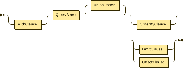
UnionOption
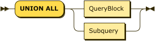
In a SQL++ query, two or more query blocks can be connected by the operator UNION ALL. The result of a UNION ALL between two query blocks contains all the items returned by the first query block, and all the items returned by the second query block. Duplicate items are not eliminated from the query result.
As in SQL, there is no ordering guarantee on the contents of the output stream. However, unlike SQL, the query language does not constrain what the data looks like on the input streams; in particular, it allows heterogeneity on the input and output streams. A type error will be raised if one of the inputs is not a collection.
When two or more query blocks are connected by UNION ALL, they can be followed by ORDER BY, LIMIT, and OFFSET clauses that apply to the UNION query as a whole. For these clauses to be meaningful, the field-names returned by the two query blocks should match. The following example shows a UNION ALL of two query blocks, with an ordering specified for the result.
In this example, a customer might be selected because he has ordered more than two different items (first query block) or because he has a high credit rating (second query block). By adding an explanatory string to each query block, the query writer can cause the output objects to be labeled to distinguish these two cases.
Example
(Q3.25a) Find customer ids for customers who have placed orders for more than two different items or who have a credit rating greater than 700, with labels to distinguish these cases.
FROM orders AS o, o.items AS i
GROUP BY o.orderno, o.custid
HAVING COUNT(*) > 2
SELECT DISTINCT o.custid AS customer_id, "Big order" AS reason

UNION ALL

FROM customers AS c
WHERE rating > 700
SELECT c.custid AS customer_id, "High rating" AS reason
ORDER BY customer_id;
Result:
[
    {
        "reason": "High rating",
        "customer_id": "C13"
    },
    {
        "reason": "Big order",
        "customer_id": "C37"
    },
    {
        "reason": "High rating",
        "customer_id": "C37"
    },
    {
        "reason": "Big order",
        "customer_id": "C41"
    }
]
If, on the other hand, you simply want a list of the customer ids and you don’t care to preserve the reasons, you can simplify your output by using SELECT VALUE, as follows:
(Q3.25b) Simplify Q3.25a to return a simple list of unlabeled customer ids.
FROM orders AS o, o.items AS i
GROUP BY o.orderno, o.custid
HAVING COUNT(*) > 2
SELECT VALUE o.custid

UNION ALL

FROM customers AS c
WHERE rating > 700
SELECT VALUE c.custid;
Result:
[
    "C37",
    "C41",
    "C13",
    "C37"
]
WITH Clause
WithClause
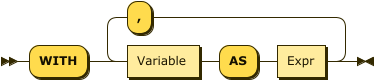
As in standard SQL, a WITH clause can be used to improve the modularity of a query. A WITH clause often contains a subquery that is needed to compute some result that is used later in the main query. In cases like this, you can think of the WITH clause as computing a "`temporary view" of the input data. The next example uses a WITH clause to compute the total revenue of each order in 2020; then the main part of the query finds the minimum, maximum, and average revenue for orders in that year.
Example
(Q3.26) Find the minimum, maximum, and average revenue among all orders in 2020, rounded to the nearest integer.
WITH order_revenue AS
    (FROM orders AS o, o.items AS i
    WHERE DATE_PART_STR(o.order_date, "year") = 2020
    GROUP BY o.orderno
    SELECT o.orderno, SUM(i.qty * i.price) AS revenue
  )
FROM order_revenue
SELECT AVG(revenue) AS average,
       MIN(revenue) AS minimum,
       MAX(revenue) AS maximum;
Result:
[
    {
        "average": 4669.99,
        "minimum": 130.45,
        "maximum": 18847.58
    }
]
WITH can be particularly useful when a value needs to be used several times in a query.
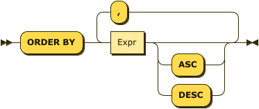
ORDER BY, LIMIT, and OFFSET Clauses
OrderbyClause
LimitClause
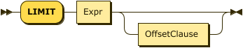
OffsetClause
The last three (optional) clauses to be processed in a query are ORDER BY, LIMIT, and OFFSET.
The ORDER BY clause is used to globally sort data in either ascending order (i.e., ASC) or descending order (i.e., DESC).
During ordering (if the NULLS modifier is not specified), MISSING and NULL are treated as being smaller than any other value if they are encountered
in the ordering key(s). MISSING is treated as smaller than NULL if both occur in the data being sorted.
The NULLS modifier determines how MISSING and NULL are ordered relative to all other values:
first (NULLS FIRST) or last (NULLS LAST). The relative order between MISSING and NULL is not affected by the NULLS modifier
(i.e. MISSING is still treated as smaller than NULL). The ordering of values of a given type is consistent with its type’s <= ordering;
the ordering of values across types is implementation-defined but stable.
The LIMIT clause is used to limit the result set to a specified maximum size.
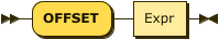
The optional OFFSET clause is used to specify a number of items in the output stream to be discarded before the query result begins.
The OFFSET can also be used as a standalone clause, without the LIMIT.
The following example illustrates use of the ORDER BY and LIMIT clauses.
Example
(Q3.27) Return the top three customers by rating.
FROM customers AS c
SELECT c.custid, c.name, c.rating
ORDER BY c.rating DESC
LIMIT 3;
Result:
[
    {
        "custid": "C13",
        "name": "T. Cody",
        "rating": 750
    },
    {
        "custid": "C37",
        "name": "T. Henry",
        "rating": 750
    },
    {
        "custid": "C25",
        "name": "M. Sinclair",
        "rating": 690
    }
]
The following example illustrates the use of OFFSET:
Example
(Q3.38) Find the customer with the third-highest credit rating.
FROM customers AS c
SELECT c.custid, c.name, c.rating
ORDER BY c.rating DESC
LIMIT 1 OFFSET 2;
Result:
[
    {
        "custid": "C25",
        "name": "M. Sinclair",
        "rating": 690
    }
]
Subqueries
Subquery

A subquery is simply a query surrounded by parentheses. In SQL++, a subquery can appear anywhere that an expression can appear. Like any query, a subquery always returns a collection, even if the collection contains only a single value or is empty. If the subquery has a SELECT clause, it returns a collection of objects. If the subquery has a SELECT VALUE clause, it returns a collection of scalar values. If a single scalar value is expected, the indexing operator [0] can be used to extract the single scalar value from the collection.
Example
(Q3.29) (Subquery in SELECT clause) For every order that includes item no. 120, find the order number, customer id, and customer name.
Here, the subquery is used to find a customer name, given a customer id. Since the outer query expects a scalar result, the subquery uses SELECT VALUE and is followed by the indexing operator [0].
FROM orders AS o, o.items AS i
WHERE i.itemno = 120
SELECT o.orderno, o.custid,
    (FROM customers AS c
     WHERE c.custid = o.custid
     SELECT VALUE c.name)[0] AS name;
Result:
[
    {
        "orderno": 1003,
        "custid": "C31",
        "name": "B. Pruitt"
    },
    {
        "orderno": 1006,
        "custid": "C41",
        "name": "R. Dodge"
    }
]
Example
(Q3.30) (Subquery in WHERE clause) Find the customer number, name, and rating of all customers whose rating is greater than the average rating.
Here, the subquery is used to find the average rating among all customers. Once again, SELECT VALUE and indexing [0] have been used to get a single scalar value.
FROM customers AS c1
WHERE c1.rating >
   (FROM customers AS c2
    SELECT VALUE AVG(c2.rating))[0]
SELECT c1.custid, c1.name, c1.rating;
Result:
[
    {
        "custid": "C13",
        "name": "T. Cody",
        "rating": 750
    },
    {
        "custid": "C25",
        "name": "M. Sinclair",
        "rating": 690
    },
    {
        "custid": "C37",
        "name": "T. Henry",
        "rating": 750
    }
]
Example
(Q3.31) (Subquery in FROM clause) Compute the total revenue (sum over items of quantity time price) for each order, then find the average, maximum, and minimum total revenue over all orders.
Here, the FROM clause expects to iterate over a collection of objects, so the subquery uses an ordinary SELECT and does not need to be indexed. You might think of a FROM clause as a "natural home" for a subquery.
FROM
   (FROM orders AS o, o.items AS i
    GROUP BY o.orderno
    SELECT o.orderno, SUM(i.qty * i.price) AS revenue
   ) AS r
SELECT AVG(r.revenue) AS average,
       MIN(r.revenue) AS minimum,
       MAX(r.revenue) AS maximum;
Result:
[
    {
        "average": 4669.99,
        "minimum": 130.45,
        "maximum": 18847.58
    }
]
Note the similarity between Q3.26 and Q3.31. This illustrates how a subquery can often be moved into a WITH clause to improve the modularity and readability of a query.
OVER Clause and Window Functions
Window functions are special functions that compute aggregate values over a "window" of input data. Like an ordinary function, a window function returns a value for every item in the input dataset. But in the case of a window function, the value returned by the function can depend not only on the argument of the function, but also on other items in the same collection. For example, a window function applied to a set of employees might return the rank of each employee in the set, as measured by salary. As another example, a window function applied to a set of items, ordered by purchase date, might return the running total of the cost of the items.
A window function call is identified by an OVER clause, which can specify three things: partitioning, ordering, and framing. The partitioning specification is like a GROUP BY: it splits the input data into partitions. For example, a set of employees might be partitioned by department. The window function, when applied to a given object, is influenced only by other objects in the same partition. The ordering specification is like an ORDER BY: it determines the ordering of the objects in each partition. The framing specification defines a "frame" that moves through the partition, defining how the result for each object depends on nearby objects. For example, the frame for a current object might consist of the two objects before and after the current one; or it might consist of all the objects before the current one in the same partition. A window function call may also specify some options that control (for example) how nulls are handled by the function.
Here is an example of a window function call:
SELECT deptno, purchase_date, item, cost,
    SUM(cost) OVER (
        PARTITION BY deptno
        ORDER BY purchase_date
        ROWS UNBOUNDED PRECEDING) AS running_total_cost
FROM purchases
ORDER BY deptno, purchase_date
This example partitions the purchases dataset by department number. Within each department, it orders the purchases by date and computes a running total cost for each item, using the frame specification ROWS UNBOUNDED PRECEDING. Note that the ORDER BY clause in the window function is separate and independent from the ORDER BY clause of the query as a whole.
The general syntax of a window function call is specified in this section. SQL++ has a set of builtin window functions, which are listed and explained in the Window Functions section of the builtin functions page. In addition, standard SQL aggregate functions such as SUM and AVG can be used as window functions if they are used with an OVER clause.
Window Function Call
WindowFunctionCall
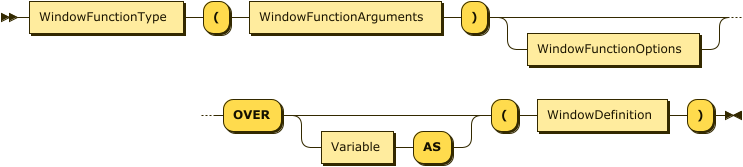
WindowFunctionType
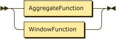
Refer to the Aggregate Functions section for a list of aggregate functions.
Refer to the Window Functions section for a list of window functions.
Window Function Arguments
WindowFunctionArguments
Refer to the Aggregate Functions section or the Window Functions section for details of the arguments for individual functions.
Window Function Options
WindowFunctionOptions

Window function options cannot be used with aggregate functions.
Window function options can only be used with some window functions, as described below.
The FROM modifier determines whether the computation begins at the first or last tuple in the window. It is optional and can only be used with the nth_value() function. If it is omitted, the default setting is FROM FIRST.
The NULLS modifier determines whether NULL values are included in the computation, or ignored. MISSING values are treated the same way as NULL values. It is also optional and can only be used with the first_value(), last_value(), nth_value(), lag(), and lead() functions. If omitted, the default setting is RESPECT NULLS.
Window Frame Variable
The AS keyword enables you to specify an alias for the window frame contents. It introduces a variable which will be bound to the contents of the frame. When using a built-in aggregate function as a window function, the function’s argument must be a subquery which refers to this alias, for example:
SELECT ARRAY_COUNT(DISTINCT (FROM alias SELECT VALUE alias.src.field))
OVER alias AS (PARTITION BY … ORDER BY …)
FROM source AS src
The alias is not necessary when using a window function, or when using a standard SQL aggregate function with the OVER clause.
Window Definition
WindowDefinition
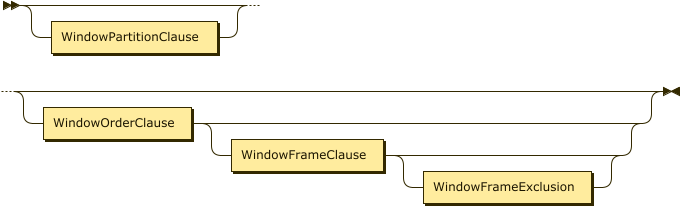
The window definition specifies the partitioning, ordering, and framing for window functions.
Window Partition Clause
WindowPartitionClause
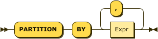
The window partition clause divides the tuples into logical partitions using one or more expressions.
This clause may be used with any window function, or any aggregate function used as a window function.
This clause is optional. If omitted, all tuples are united in a single partition.
Window Order Clause
WindowOrderClause
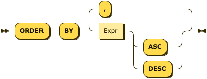
The window order clause determines how tuples are ordered within each partition. The window function works on tuples in the order specified by this clause.
This clause may be used with any window function, and most aggregate functions — refer to the descriptions of individual functions for more details.
This clause is optional. If omitted, all tuples are considered peers, i.e. their order is tied. When tuples in the window partition are tied, each window function behaves differently.
-
The
row_number()function returns a distinct number for each tuple. If tuples are tied, the results may be unpredictable. -
The
rank(),dense_rank(),percent_rank(), andcume_dist()functions return the same result for each tuple. -
For other functions, if the window frame is defined by
ROWS, the results may be unpredictable. If the window frame is defined byRANGEorGROUPS, the results are same for each tuple.
This clause does not guarantee the overall order of the query results. To guarantee the order of the final results, use the query ORDER BY clause.
|
Window Frame Clause
WindowFrameClause
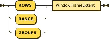
The window frame clause defines the window frame. It can be used with some window functions and most aggregate functions — refer to the descriptions of individual functions for more details. It is optional and allowed only when the window order clause is present.
-
If this clause is omitted and there is no window order clause, the window frame is the entire partition.
-
If this clause is omitted but there is a window order clause, the window frame becomes all tuples in the partition preceding the current tuple and its peers — the same as
RANGE BETWEEN UNBOUNDED PRECEDING AND CURRENT ROW.
The window frame can be defined in the following ways:
-
ROWS: Counts the exact number of tuples within the frame. If window ordering doesn’t result in unique ordering, the function may produce unpredictable results. You can add a unique expression or more window ordering expressions to produce unique ordering. -
RANGE: Looks for a value offset within the frame. The function produces deterministic results. -
GROUPS: Counts all groups of tied rows within the frame. The function produces deterministic results.
If this clause uses RANGE with either Expr PRECEDING or Expr FOLLOWING, the window order clause must have only a single ordering term.
The ordering term expression must evaluate to a number.
If these conditions are not met, the window frame will be empty, which means the window function will return its default value: in most cases this is null, except for strict_count() or array_count(), whose default value is 0. This restriction does not apply when the window frame uses ROWS or GROUPS.
|
The RANGE window frame is commonly used to define window frames based
on date or time.
If you want to use RANGE with either Expr PRECEDING or Expr FOLLOWING, and you want to use an ordering expression based on date or time, the expression in Expr PRECEDING or Expr FOLLOWING must use a data type that can be added to the ordering expression.
|
Window Frame Extent
WindowFrameExtent
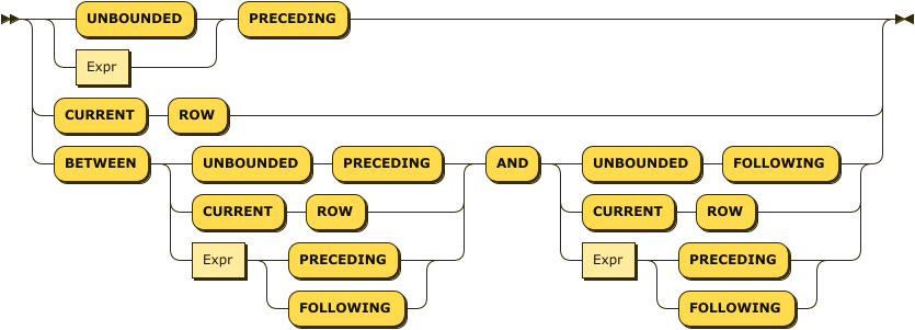
The window frame extent clause specifies the start point and end point of the window frame.
The expression before AND is the start point and the expression after AND is the end point.
If BETWEEN is omitted, you can only specify the start point; the end point becomes CURRENT ROW.
The window frame end point can’t be before the start point. If this clause violates this restriction explicitly, an error will result. If it violates this restriction implicitly, the window frame will be empty, which means the window function will return its default value: in most cases this is null, except for strict_count() or
array_count(), whose default value is 0.
Window frame extents that result in an explicit violation are:
-
BETWEEN CURRENT ROW ANDExprPRECEDING -
BETWEENExprFOLLOWING ANDExprPRECEDING -
BETWEENExprFOLLOWING AND CURRENT ROW
Window frame extents that result in an implicit violation are:
-
BETWEEN UNBOUNDED PRECEDING ANDExprPRECEDING— if Expr is too high, some tuples may generate an empty window frame. -
BETWEENExprPRECEDING ANDExprPRECEDING— if the second Expr is greater than or equal to the first Expr, all result sets will generate an empty window frame. -
BETWEENExprFOLLOWING ANDExprFOLLOWING— if the first Expr is greater than or equal to the second Expr, all result sets will generate an empty window frame. -
BETWEENExprFOLLOWING AND UNBOUNDED FOLLOWING— if Expr is too high, some tuples may generate an empty window frame. -
If the window frame exclusion clause is present, any window frame specification may result in empty window frame.
The Expr must be a positive constant or an expression that evaluates as a positive number. For ROWS or GROUPS, the Expr must be an integer.
Window Frame Exclusion
WindowFrameExclusion
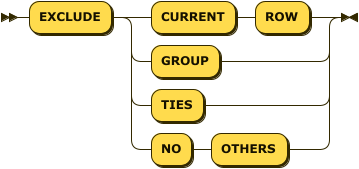
The window frame exclusion clause enables you to exclude specified tuples from the window frame.
This clause can be used with all aggregate functions and some window functions — refer to the descriptions of individual functions for more details.
This clause is allowed only when the window frame clause is present.
This clause is optional. If this clause is omitted, the default is no exclusion — the same as EXCLUDE NO OTHERS.
-
EXCLUDE CURRENT ROW: If the current tuple is still part of the window frame, it is removed from the window frame. -
EXCLUDE GROUP: The current tuple and any peers of the current tuple are removed from the window frame. -
EXCLUDE TIES: Any peers of the current tuple, but not the current tuple itself, are removed from the window frame. -
EXCLUDE NO OTHERS: No additional tuples are removed from the window frame.
If the current tuple is already removed from the window frame, then it remains removed from the window frame.
Differences from SQL-92
SQL++ offers the following additional features beyond SQL-92:
-
Fully composable and functional: A subquery can iterate over any intermediate collection and can appear anywhere in a query.
-
Schema-free: The query language does not assume the existence of a static schema for any data that it processes.
-
Correlated
FROMterms: A right-sideFROMterm expression can refer to variables defined byFROMterms on its left. -
Powerful
GROUP BY: In addition to a set of aggregate functions as in standard SQL, the groups created by theGROUP BYclause are directly usable in nested queries and/or to obtain nested results. -
Generalized
SELECTclause: ASELECTclause can return any type of collection, while in SQL-92, aSELECTclause has to return a (homogeneous) collection of objects.
The following matrix is a quick "SQL-92 compatibility cheat sheet" for SQL++.
| Feature | SQL++ | SQL-92 | Why different? |
|---|---|---|---|
SELECT * |
Returns nested objects |
Returns flattened concatenated objects |
Nested collections are 1st class citizens |
SELECT list |
order not preserved |
order preserved |
Fields in a JSON object are not ordered |
Subquery |
Returns a collection |
The returned collection is cast into a scalar value if the subquery appears in a SELECT list or on one side of a comparison or as input to a function |
Nested collections are 1st class citizens |
LEFT OUTER JOIN |
Fills in |
Fills in |
"Absence" is more appropriate than "unknown" here |
UNION ALL |
Allows heterogeneous inputs and output |
Input streams must be UNION-compatible and output field names are drawn from the first input stream |
Heterogenity and nested collections are common |
IN constant_expr |
The constant expression has to be an array or multiset, i.e., [..,..,…] |
The constant collection can be represented as comma-separated items in a paren pair |
Nested collections are 1st class citizens |
String literal |
Double quotes or single quotes |
Single quotes only |
Double quoted strings are pervasive in JSON |
Delimited identifiers |
Backticks |
Double quotes |
Double quoted strings are pervasive in JSON |
The following SQL-92 features are not implemented yet. However, SQL++ does not conflict with these features:
-
CROSS JOIN, NATURAL JOIN, UNION JOIN
-
FULL OUTER JOIN
-
INTERSECT, EXCEPT, UNION with set semantics
-
CAST expression
-
ALL and SOME predicates for linking to subqueries
-
UNIQUE predicate (tests a collection for duplicates)
-
MATCH predicate (tests for referential integrity)
-
Row and Table constructors
-
Preserved order for expressions in a SELECT list