Admin basics
A newer version of this software is available
You are viewing the documentation for an older version of this software. To find the documentation for the current version, visit the Couchbase documentation home page.
This chapter covers everything on the Administration of a Couchbase Sever cluster. Administration is supported through three primary methods:
-
Couchbase Web Console
Couchbase includes a built-in web server and administration interface that provides access to the administration and statistic information for your cluster.
For more information, see the Couchbase Web Console.
-
Command-line Toolkit
Provided within the Couchbase package are a number of command-line tools that allow you to communicate and control your Couchbase cluster.
For more information, see the Command-line interface.
-
Couchbase REST API
Couchbase Server includes a RESTful API that enables any tool capable of communicating over HTTP to administer and monitor a Couchbase cluster.
For more information, see the REST API.
-
Best Practices
For information on deploying and building your Couchbase Server cluster, see Best Practices and in particular, Deployment Strategies.
If you already have an application that uses the Memcached protocol then you can start using your Couchbase Server immediately. If so, you can simply point your application to this server like you would any other memcached server. No code changes or special libraries are needed, and the application will behave exactly as it would against a standard memcached server. Without the client knowing anything about it, the data is being replicated, persisted, and the cluster can be expanded or contracted completely transparently.
If you do not already have an application, then you should investigate one of the available Couchbase client libraries to connect to your server and start storing and retrieving information. For more information, see Couchbase SDKs.
Couchbase data files
By default, Couchbase Server stores data files under the following paths:
| Platform | Directory |
|---|---|
| Linux | /opt/couchbase/var/lib/couchbase/data
|
| Windows | C:\Program Files\couchbase\server\var\lib\couchbase\data
|
| Mac OS X | ~/Library/Application Support/Couchbase/var/lib/couchbase/data
|
This path can be changed for each node at setup either via the Web UI setup wizard, using the REST API or using the Couchbase CLI:
Warning
Changing the data path for a node that is already part of a cluster will permanently delete the data stored.
Linux:
> couchbase-cli node-init -c node_IP:8091 \
    --node-init-data-path=new_path \
    -u user -p password
Windows:
> couchbase-cli node-init -c \
    node_IP:8091 --node-init-data-path=new_path \
    -u user -p password
Note
When using the command line tool, you cannot change the data file and index file path settings individually. If you need to configure the data file and index file paths individually, use the REST API. For more information, see Configuring Index Path for a Node.
Once a node or cluster has already been setup and is storing data, you cannot change the path while the node is part of a running cluster. You must take the node out of the cluster then follow the steps below:
Change the path on a running node either via the REST API or using the Couchbase CLI (commands above). This change will not actually take effect until the node is restarted. For more information about using a REST API request for ejecting nodes from clusters, see Removing a Node from a Cluster.
Shut the node down.
Copy all the data files from their original location into the new location.
Start the service again and monitor the “warmup” of the data.
Server startup and shutdown
The packaged installations of Couchbase Server include support for automatically starting and stopping Couchbase Server using the native boot and shutdown mechanisms.
For information on starting and stopping Couchbase Server, see the different platform-specific links:
Startup and shutdown on Linux
On Linux, Couchbase Server is installed as a standalone application with support
for running as a background (daemon) process during startup through the use of a
standard control script, /etc/init.d/couchbase-server. The startup script is
automatically installed during installation from one of the Linux packaged
releases (Debian/Ubuntu or Red Hat/CentOS). By default Couchbase Server is
configured to be started automatically at run levels 2, 3, 4, and 5, and
explicitly shutdown at run levels 0, 1 and 6.
To manually start Couchbase Server using the startup/shutdown script:
> sudo /etc/init.d/couchbase-server start
To manually stop Couchbase Server using the startup/shutdown script:
> sudo /etc/init.d/couchbase-server stop
Startup and shutdown on Windows
On Windows, Couchbase Server is installed as a Windows service. You can use the
Services tab within the Windows Task Manager to start and stop Couchbase
Server.
Note
You will need Power User or Administrator privileges or have been separately granted the rights to manage services to start and stop Couchbase Server.
By default, the service should start automatically when the machine boots. To
manually start the service, open the Windows Task Manager and choose the
Services tab, or select the Start, choose Run and then type Services.msc
to open the Services management console.
Once open, find the CouchbaseServer service, right-click and then choose to
Start or Stop the service as appropriate. You can also alter the configuration
so that the service is not automatically started during boot.
Alternatively, you can start and stop the service from the command-line, either
by using the system net command. For example, to start Couchbase Server:
> net start CouchbaseServer
To stop Couchbase Server:
> net stop CouchbaseServer
Start and Stop scripts are also provided in the standard Couchbase Server
installation in the bin directory. To start the server using this script:
> C:\Program Files\Couchbase\Server\bin\service_start.bat
To stop the server using the supplied script:
> C:\Program Files\Couchbase\Server\bin\service_stop.bat
Startup and shutdown on Mac OS X
On Mac OS X, Couchbase Server is supplied as a standard application. You can start Couchbase Server by double clicking on the application. Couchbase Server runs as a background application which installs a menu bar item through which you can control the server.
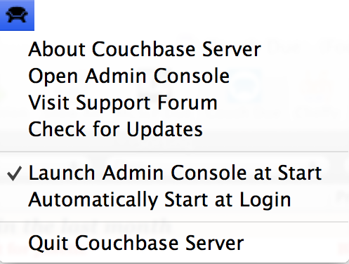
The individual menu options perform the following actions:
-
About CouchbaseOpens a standard About dialog containing the licensing and version information for the Couchbase Server installed.
-
Open Admin ConsoleOpens the Web Administration Console in your configured default browser.
-
Visit Support ForumOpens the Couchbase Server support forum within your default browser at the Couchbase website where you can ask questions to other users and Couchbase developers.
-
Check for UpdatesChecks for updated versions of Couchbase Server. This checks the currently installed version against the latest version available at Couchbase and offers to download and install the new version. If a new version is available, you will be presented with a dialog containing information about the new release.
If a new version is available, you can choose to skip the update, notify the existence of the update at a later date, or to automatically update the software to the new version.
If you choose the last option, the latest available version of Couchbase Server will be downloaded to your machine, and you will be prompted to allow the installation to take place. Installation will shut down your existing Couchbase Server process, install the update, and then restart the service once the installation has been completed.
Once the installation has been completed you will be asked whether you want to automatically update Couchbase Server in the future.
Note
Using the update service also sends anonymous usage data to Couchbase on the current version and cluster used in your organization. This information is used to improve our service offerings.
You can also enable automated updates by selecting the
Automatically download
and install updates in the future
checkbox. -
Launch Admin Console at StartIf this menu item is checked, then the Web Console for administrating Couchbase Server will be opened whenever the Couchbase Server is started. Selecting the menu item will toggle the selection.
-
Automatically Start at LoginIf this menu item is checked, then Couchbase Server will be automatically started when the Mac OS X machine starts. Selecting the menu item will toggle the selection.
-
Quit CouchbaseSelecting this menu option will shut down your running Couchbase Server, and close the menu bar interface. To restart, you must open the Couchbase Server application from the installation folder.
Architecture and concepts
In order to understand the structure and layout of Couchbase Server, you first need to understand the different components and systems that make up both an individual Couchbase Server instance, and the components and systems that work together to make up the Couchbase Cluster as a whole.
The following section provides key information and concepts that you need to understand the fast and elastic nature of the Couchbase Server database, and how some of the components work together to support a highly available and high performance database.
Nodes and clusters
Couchbase Server can be used either in a standalone configuration, or in a cluster configuration where multiple Couchbase Servers are connected together to provide a single, distributed, data store.
In this description:
-
Couchbase Server or Node
A single instance of the Couchbase Server software running on a machine, whether a physical machine, virtual machine, EC2 instance or other environment.
All instances of Couchbase Server are identical, provide the same functionality, interfaces and systems, and consist of the same components.
-
Cluster
A cluster is a collection of one ore more instances of Couchbase Server that are configured as a logical cluster. All nodes within the cluster are identical and provide the same functionality. Each node is capable of managing the cluster and each node can provide aggregate statistics and operational information about the cluster. User data is stored across the entire cluster through the vBucket system.
Clusters operate in a completely horizontal fashion. To increase the size of a cluster, you add another node. There are no parent/child relationships or hierarchical structures involved. This means that Couchbase Server scales linearly, both in terms of increasing the storage capacity and the performance and scalability.
Cluster Manager
Every node within a Couchbase Cluster includes the Cluster Manager component. The Cluster Manager is responsible for the following within a cluster:
Cluster management
Node administration
Node monitoring
Statistics gathering and aggregation
Run-time logging
Multi-tenancy
Security for administrative and client access
Client proxy service to redirect requests
Access to the Cluster Manager is provided through the administration interface (see Administration Tools ) on a dedicated network port, and through dedicated network ports for client access. Additional ports are configured for inter-node communication.
Data storage
Couchbase Server provides data management services using buckets ; these are isolated virtual containers for data. A bucket is a logical grouping of physical resources within a cluster of Couchbase Servers. They can be used by multiple client applications across a cluster. Buckets provide a secure mechanism for organizing, managing, and analyzing data storage resources.
There are two types of data bucket in Couchbase Server: 1) memcached buckets, and 2) couchbase buckets. The two different types of buckets enable you to store data in-memory only, or to store data in-memory as well as on disk for added reliability. When you set up Couchbase Server you can choose what type of bucket you need in your implementation:
| Bucket Type | Description |
|---|---|
| Couchbase | Provides highly-available and dynamically reconfigurable distributed data storage, providing persistence and replication services. Couchbase buckets are 100% protocol compatible with, and built in the spirit of, the memcached open source distributed key-value cache. |
| Memcached | Provides a directly-addressed, distributed (scale-out), in-memory, key-value cache. Memcached buckets are designed to be used alongside relational database technology – caching frequently-used data, thereby reducing the number of queries a database server must perform for web servers delivering a web application. |
The different bucket types support different capabilities. Couchbase-type buckets provide a highly-available and dynamically reconfigurable distributed data store. Couchbase-type buckets survive node failures and allow cluster reconfiguration while continuing to service requests. Couchbase-type buckets provide the following core capabilities.
| Capability | Description |
|---|---|
| Caching | Couchbase buckets operate through RAM. Data is kept in RAM and persisted down to disk. Data will be cached in RAM until the configured RAM is exhausted, when data is ejected from RAM. If requested data is not currently in the RAM cache, it will be loaded automatically from disk. |
| Persistence | Data objects can be persisted asynchronously to hard-disk resources from memory to provide protection from server restarts or minor failures. Persistence properties are set at the bucket level. |
| Replication | A configurable number of replica servers can receive copies of all data objects in the Couchbase-type bucket. If the host machine fails, a replica server can be promoted to be the host server, providing high availability cluster operations via failover. Replication is configured at the bucket level. |
| Rebalancing | Rebalancing enables load distribution across resources and dynamic addition or removal of buckets and servers in the cluster. |
| Capability | memcached Buckets | Couchbase Buckets |
|---|---|---|
| Item Size Limit | 1 MByte | 20 MByte |
| Persistence | No | Yes |
| Replication | No | Yes |
| Rebalance | No | Yes |
| Statistics | Limited set for in-memory stats | Full suite |
| Client Support | Memcached, should use Ketama consistent hashing | Full Smart Client Support |
| XDCR | No | Yes |
| Backup | No | Yes |
| Tap/DCP | No | Yes |
| Encrypted Data Access | No | Yes |
There are three bucket interface types that can be be configured:
-
The default bucket
The default bucket is a Couchbase bucket that always resides on port 11211 and is a non-SASL authenticating bucket. When Couchbase Server is first installed this bucket is automatically set up during installation. This bucket may be removed after installation and may also be re-added later, but when re-adding a bucket named “default”, the bucket must be place on port 11211 and must be a non-SASL authenticating bucket. A bucket not named default may not reside on port 11211 if it is a non-SASL bucket. The default bucket may be reached with a vBucket aware smart client, an ASCII client or a binary client that doesn’t use SASL authentication.
-
Non-SASL buckets
Non-SASL buckets may be placed on any available port with the exception of port 11211 if the bucket is not named “default”. Only one Non-SASL bucket may placed on any individual port. These buckets may be reached with a vBucket aware smart client, an ASCII client or a binary client that doesn’t use SASL authentication
-
SASL buckets
SASL authenticating Couchbase buckets may only be placed on port 11211 and each bucket is differentiated by its name and password. SASL bucket may not be placed on any other port beside 11211. These buckets can be reached with either a vBucket aware smart client or a binary client that has SASL support. These buckets cannot be reached with ASCII clients.
Smart clients discover changes in the cluster using the Couchbase Management REST API. Buckets can be used to isolate individual applications to provide multi-tenancy, or to isolate data types in the cache to enhance performance and visibility. Couchbase Server allows you to configure different ports to access different buckets, and gives you the option to access isolated buckets using either the binary protocol with SASL authentication, or the ASCII protocol with no authentication
Couchbase Server enables you to use and mix different types of buckets, Couchbase and Memcached, as appropriate in your environment. Buckets of different types still share the same resource pool and cluster resources. Quotas for RAM and disk usage are configurable per bucket so that resource usage can be managed across the cluster. Quotas can be modified on a running cluster so that administrators can reallocate resources as usage patterns or priorities change over time.
For more information about creating and managing buckets, see the following resources:
Bucket RAM Quotas: see RAM Quotas.
Creating and Managing Buckets with Couchbase Web Console: see Viewing Data Buckets.
Creating and Managing Buckets with Couchbase REST API: see Managing Buckets.
Creating and Managing Buckets with Couchbase CLI (Command-Line Tool): see couchbase-cli tool.
RAM quotas
RAM is allocated to Couchbase Server in two different configurable quantities,
the Server Quota and Bucket Quota.
-
Server quota
The Server Quota is the RAM that is allocated to the server when Couchbase Server is first installed. This sets the limit of RAM allocated by Couchbase for caching data for all buckets and is configured on a per-node basis. The Server Quota is initially configured in the first server in your cluster is configured, and the quota is identical on all nodes. For example, if you have 10 nodes and a 16GB Server Quota, there is 160GB RAM available across the cluster. If you were to add two more nodes to the cluster, the new nodes would need 16GB of free RAM, and the aggregate RAM available in the cluster would be 192GB.
-
Bucket quota
The Bucket Quota is the amount of RAM allocated to an individual bucket for caching data. Bucket quotas are configured on a per-node basis, and is allocated out of the RAM defined by the Server Quota. For example, if you create a new bucket with a Bucket Quota of 1GB, in a 10 node cluster there would be an aggregate bucket quota of 10GB across the cluster. Adding two nodes to the cluster would extend your aggregate bucket quota to 12GB.
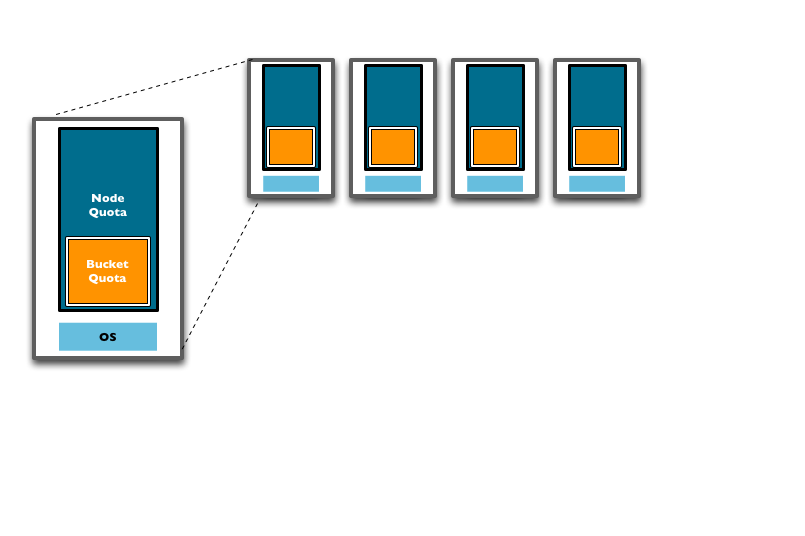
From this description and diagram, you can see that adding new nodes to the cluster expands the overall RAM quota, and the bucket quota, increasing the amount of information that can be kept in RAM.
The Bucket Quota is used by the system to determine when data should be ejected from memory. Bucket Quotas are dynamically configurable within the limit of your Server Quota, and enable you to individually control the caching of information in memory on a per bucket basis. You can therefore configure different buckets to cope with your required caching RAM allocation requirements.
The Server Quota is also dynamically configurable, but care must be taken to ensure that the nodes in your cluster have the available RAM to support your chosen RAM quota configuration.
vBuckets
A vBucket is defined as the owner of a subset of the key space of a Couchbase cluster. These vBuckets are used to allow information to be distributed effectively across the cluster. The vBucket system is used both for distributing data, and for supporting replicas (copies of bucket data) on more than one node.
Clients access the information stored in a bucket by communicating directly with the node responsible for the corresponding vBucket. This direct access enables clients to communicate with the node storing the data, rather than using a proxy or redistribution architecture. The result is abstracting the physical topology from the logical partitioning of data. This architecture is what gives Couchbase Server the elasticity.
This architecture differs from the method used by memcached, which uses
client-side key hashes to determine the server from a defined list. This
requires active management of the list of servers, and specific hashing
algorithms such as Ketama to cope with changes to the topology. The structure is
also more flexible and able to cope better with changes than the typical sharding
arrangement used in an RDBMS environment.
Note
vBuckets are not a user-accessible component, but they are a critical component of Couchbase Server and are vital to the availability support and the elastic nature.
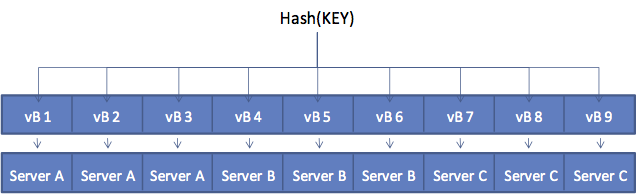
Every document ID belongs to a vBucket. A mapping function is used to calculate the vBucket in which a given document belongs. In Couchbase Server, that mapping function is a hashing function that takes a document ID as input and outputs a vBucket identifier. Once the vBucket identifier has been computed, a table is consulted to lookup the server that “hosts” that vBucket. The table contains one row per vBucket, pairing the vBucket to its hosting server. A server appearing in this table can be (and usually is) responsible for multiple vBuckets.
The following diagram shows how the Key to Server mapping (vBucket map) works. There
are three servers in the cluster. A client wants to look up ( get ) the value
of KEY. The client first hashes the key to calculate the vBucket which owns KEY.
In this example, the hash resolves to vBucket 8 ( vB8 ) By examining the
vBucket map, the client determines Server C hosts vB8. The get operation is
sent directly to Server C.
After some period of time, there is a need to add a server to the cluster. A new node, Server D is added to the cluster and the vBucket Map is updated.
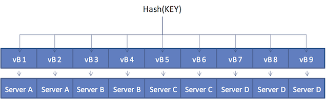
Note
The vBucket map is updated during the rebalance operation; the updated map is then sent to all the cluster participants, including the other nodes, any connected "smart" clients, and the Moxi proxy service.
Within the new four-node cluster model, when a client again wants to get the
value of KEY, the hashing algorithm still resolves to vBucket 8 ( vB8 ).
The new vBucket map however now maps that vBucket to Server D. The client now
communicates directly with Server D to obtain the information.
Caching layer
The architecture of Couchbase Server includes a built-in caching layer. This caching layer acts as a central part of the server and provides very rapid reads and writes of data. Other database solutions read and write data from disk, which results in much slower performance. One alternative approach is to install and manage a caching layer as a separate component which will work with a database. This approach also has drawbacks because the burden of managing transfer of data between caching layer and database and the burden managing the caching layer results in significant custom code and effort.
In contrast Couchbase Server automatically manages the caching layer and coordinates with disk space to ensure that enough cache space exists to maintain performance. Couchbase Server automatically places items that come into the caching layer into disk queue so that it can write these items to disk. If the server determines that a cached item is infrequently used, it can remove it from RAM to free space for other items. Similarly the server can retrieve infrequently-used items from disk and store them into the caching layer when the items are requested. So the entire process of managing data between the caching layer and data persistence layer is handled entirely by server. In order provide the most frequently-used data while maintaining high performance, Couchbase Server manages a working set of your entire information; this set consists of the all data you most frequently access and is kept in RAM for high performance.
Couchbase automatically moves data from RAM to disk asynchronously in the background in order to keep frequently used information in memory, and less frequently used data on disk. Couchbase constantly monitors the information accessed by clients, and decides how to keep the active data within the caching layer. Data is ejected to disk from memory in the background while the server continues to service active requests. During sequences of high writes to the database, clients will be notified that the server is temporarily out of memory until enough items have been ejected from memory to disk. The asynchronous nature and use of queues in this way enables reads and writes to be handled at a very fast rate, while removing the typical load and performance spikes that would otherwise cause a traditional RDBMS to produce erratic performance.
When the server stores data on disk and a client requests the data, it sends an
individual document ID then the server determines whether the information exists
or not. Couchbase Server does this with metadata structures. The metadata
holds information about each document in the database and this information is
held in RAM. This means that the server can always return a ‘document ID not
found’ response for an invalid document ID or it can immediately return the data
from RAM, or return it after it fetches it from disk.
Disk storage
For performance, Couchbase Server mainly stores and retrieves information for clients using RAM. At the same time, Couchbase Server will eventually store all data to disk to provide a higher level of reliability. If a node fails and you lose all data in the caching layer, you can still recover items from disk. We call this process of disk storage eventual persistence since the server does not block a client while it writes to disk, rather it writes data to the caching layer and puts the data into a disk write queue to be persisted to disk. Disk persistence enables you to perform backup and restore operations, and enables you to grow your datasets larger than the built-in caching layer. For more information, see Ejection, Eviction and Working Set Management.
When the server identifies an item that needs to be loaded from disk because it is not in active memory, the process is handled by a background process that processes the load queue and reads the information back from disk and into memory. The client is made to wait until the data has been loaded back into memory before the information is returned.
Multiple readers and writers
Multiple readers and writers are supported to persist data onto disk. For earlier versions of Couchbase Server, each server instance had only single disk reader and writer threads. Disk speeds have now increased to the point where single read/write threads do not efficiently keep up with the speed of disk hardware. The other problem caused by single read/writes threads is that if you have a good portion of data on disk and not RAM, you can experience a high level of cache misses when you request this data. In order to utilize increased disk speeds and improve the read rate from disk, we now provide multi-threaded readers and writers so that multiple processes can simultaneously read and write data on disk:
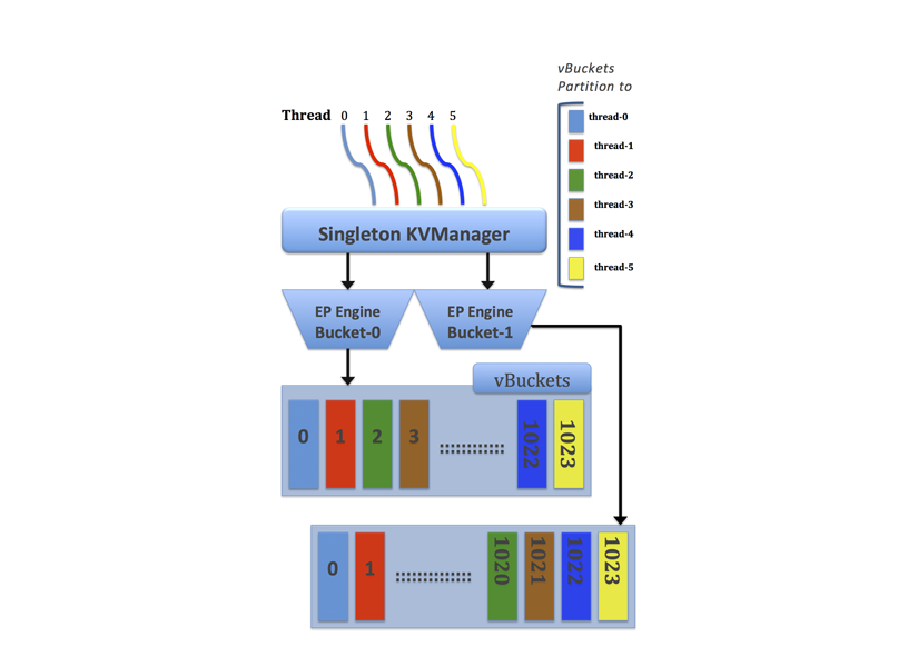
This multi-threaded engine includes additional synchronization among threads that are accessing the same data cache to avoid conflicts. To maintain performance while avoiding conflicts over data we use a form of locking between threads as well as thread allocation among vBuckets with static partitioning. When Couchbase Server creates multiple reader and writer threads, the server assesses a range of vBuckets for each thread and assigns each thread exclusively to certain vBuckets. With this static thread coordination, the server schedules threads so that only a single reader and single writer thread can access the same vBucket at any given time. We show this in the image above with six pre-allocated threads and two data Buckets. Each thread has the range of vBuckets that is statically partitioned for read and write access.
For information about configuring this option, see Using Multi- Readers and Writers.
Document deletion from disk
For Couchbase Server will never delete entire items from disk unless a client explicitly deletes the item from the database or the expiration value for the item is reached. The ejection mechanism removes an item from RAM, while keeping a copy of the key and metadata for that document in RAM and also keeping copy of that document on disk. For more information about document expiration and deletion, see Couchbase Developer Guide, About Document Expiration.
Tombstone purging
Couchbase Server and other distributed databases maintain tombstones in order to provide eventual consistency between nodes and between clusters. Tombstones are records of expired or deleted items and they include the key for the item as well as metadata. Couchbase Server stores the key plus several bytes of metadata per deleted item in two structures per node. With millions of mutations, the space taken up by tombstones can grow quickly. This is especially the case if you have a large number of deletions or expired documents.
You can now configure the Metadata Purge Interval which sets how frequently a node will permanently purge metadata on deleted and expired items. This new setting will run as part of auto-compaction. This helps reduce the storage requirement by roughly 3x times lower than before and also frees up space much faster:
In Web Console, see Using Web Console, Enabling Auto-Compaction.
You can also change this interval via REST, see the REST API, Setting Auto-Compaction.
Ejection, eviction and working set management
Ejection is a process automatically performed by Couchbase Server; it is the process of removing data from RAM to provide room for frequently-used items. When Couchbase Server ejects information, it works in conjunction with the disk persistence system to ensure that data in RAM has been persisted to disk and can be safely retrieved back into RAM if the item is requested. The process that Couchbase Server performs to free space in RAM, and to ensure the most-used items are still available in RAM is also known as working set management.
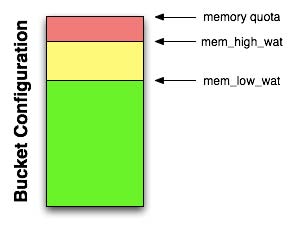
In addition to memory quota for the caching layer, there are two watermarks the
engine uses to determine when it is necessary to start persisting more data
to disk. These are mem_low_wat and mem_high_wat.
As the caching layer becomes full of data, eventually the mem_low_wat is
passed. At this time, no action is taken. As data continues to load, it will
eventually reach mem_high_wat. At this point a background job is scheduled to
ensure items are migrated to disk and the memory is then available for other
Couchbase Server items. This job runs until measured memory reaches
mem_low_wat. If the rate of incoming items is faster than the migration of
items to disk, the system may return errors indicating there is not enough
space. This will continue until there is available memory. The process of
removing data from the caching to make way for the actively used information is
called ejection, and is controlled automatically through thresholds set on
each configured bucket in your Couchbase Server Cluster.
Some of you may be using only memcached buckets with Couchbase Server; in this case the server provides only a caching layer as storage and no data persistence on disk. If your server runs out of space in RAM, it will evict items from RAM on a least recently used basis (LRU). Eviction means the server will remove the key, metadata and all other data for the item from RAM. After eviction, the item is irretrievable.
For more detailed technical information about ejection and working set management, including any administrative tasks which impact this process, see Ejection and Working Set Management.
Expiration
Each document stored in the database has an optional expiration value (TTL, time to live). The default is for there to be no expiration, i.e. the information will be stored indefinitely. The expiration can be used for data that naturally has a limited life that you want to be automatically deleted from the entire database.
The expiration value is user-specified on a per document basis at the point when the object is created, updated, or changed through the Couchbase SDK. If you want an object to expire before 30 days, you can provide a TTL in seconds, or as Unix epoch time. If you want an object to expire sometime after 30 days, you must provide a TTL in Unix epoch time; for instance, 1 095 379 198 indicates the seconds since 1970."
Typical uses for an expiration value include web session data, where you want the actively stored information to be removed from the system if the user activity has stopped and not been explicitly deleted. The data will time out and be removed from the system, freeing up RAM and disk for more active data.
Server warmup
Anytime you restart the Couchbase Server, or when you restore data to a server instance, the server must undergo a warmup process before it can handle requests for the data. During warmup the server loads data from disk into RAM; after the warmup process completes, the data is available for clients to read and write. Depending on the size and configuration of your system and the amount of data persisted in your system, server warmup may take some time to load all of the data into memory.
Couchbase Server provides a more optimized warmup process; instead of loading data sequentially from disk into RAM, it divides the data to be loaded and handles it in multiple phases. Couchbase Server is also able to begin serving data before it has actually loaded all the keys and data from vBuckets. For more technical details about server warmup and how to manage server warmup, see Handling Server Warmup.
Rebalancing
The way data is stored within Couchbase Server is through the distribution
offered by the vBucket structure. If you want to expand or shrink your Couchbase
Server cluster then the information stored in the vBuckets needs to be
redistributed between the available nodes, with the corresponding vBucket map
updated to reflect the new structure. This process is called rebalancing.
Rebalancing is an deliberate process that you need to initiate manually when the structure of your cluster changes. The rebalance process changes the allocation of the vBuckets used to store the information and then physically moves the data between the nodes to match the new structure.
The rebalancing process can take place while the cluster is running and servicing requests. Clients using the cluster read and write to the existing structure with the data being moved in the background between nodes. Once the moving process has been completed, the vBucket map is updated and communicated to the smart clients and the proxy service (Moxi).
The result is that the distribution of data across the cluster has been rebalanced, or smoothed out, so that the data is evenly distributed across the database, taking into account the data and replicas of the data required to support the system.
Replicas and replication
In addition to distributing information across the cluster for even data distribution and cluster performance, you can also establish replica vBuckets within a single Couchbase cluster.
A copy of data from one bucket, known as a source will be copied to a destination, which we also refer to as the replica, or replica vBucket. The node that contains the replica vBucket is also referred to as the replica node while the node containing original data to be replicated is called a source node. Distribution of replica data is handled in the same way as data at a source node; portions of replica data will be distributed around the cluster to prevent a single point of failure.
After Couchbase has stored replica data at a destination node, the data will also be placed in a queue to be persisted on disk at that destination node. For more technical details about data replication within Couchbase clusters, or to learn about any configurations for replication, see Handling Replication within a Cluster.
You are also able to perform replication between two Couchbase clusters. This is known as cross datacenter replication (XDCR) and can provide a copy of your data at a cluster which is closer to your users, or to provide the data in case of disaster recovery. For more information about replication between clusters via XDCR see Cross Datacenter Replication (XDCR).
Failover
Information is distributed around a cluster using a series of replicas. For
Couchbase buckets you can configure the number of replicas (complete copies of
the data stored in the bucket) that should be kept within the Couchbase Server
Cluster.
In the event of a failure in a server (either due to transient failure, or for
administrative purposes), you can use a technique called failover to indicate
that a node within the Couchbase Cluster is no longer available, and that the
replica vBuckets for the server are enabled.
The failover process contacts each server that was acting as a replica and updates the internal table that maps client requests for documents to an available server.
Failover can be performed manually, or you can use the built-in automatic failover that reacts after a preset time when a node within the cluster becomes unavailable.
For more information, see Failover nodes.
TAP
The TAP protocol is an internal part of the Couchbase Server system and is used in a number of different areas to exchange data throughout the system. TAP provides a stream of data of the changes that are occurring within the system.
TAP is used during replication, to copy data between vBuckets used for replicas. It is also used during the rebalance procedure to move data between vBuckets and redistribute the information across the system.
Client interface
Within Couchbase Server, the techniques and systems used to get information into and out of the database differ according to the level and volume of data that you want to access. The different methods can be identified according to the base operations of Create, Retrieve, Update and Delete:
-
Create
Information is stored into the database using the memcached protocol interface to store a value against a specified key. Bulk operations for setting the key/value pairs of a large number of documents at the same time are available, and these are more efficient than multiple smaller requests.
The value stored can be any binary value, including structured and unstructured strings, serialized objects (from the native client language), native binary data (for example, images or audio). For use with the Couchbase Server View engine, information must be stored using the JavaScript Object Notation (JSON) format, which structures information as a object with nested fields, arrays, and scalar datatypes.
-
Retrieve
To retrieve information from the database, there are two methods available:
-
By Key
If you know the key used to store a particular value, then you can use the memcached protocol (or an appropriate memcached compatible client-library) to retrieve the value stored against a specific key. You can also perform bulk operations
-
By View
If you do not know the key, you can use the View system to write a view that outputs the information you need. The view generates one or more rows of information for each JSON object stored in the database. The view definition includes the keys (used to select specific or ranges of information) and values. For example, you could create a view on contact information that outputs the JSON record by the contact’s name, and with a value containing the contacts address. Each view also outputs the key used to store the original object. If the view doesn’t contain the information you need, you can use the returned key with the memcached protocol to obtain the complete record.
-
-
Update
To update information in the database, you must use the memcached protocol interface. The memcached protocol includes functions to directly update the entire contents, and also to perform simple operations, such as appending information to the existing record, or incrementing and decrementing integer values.
-
Delete
To delete information from Couchbase Server you need to use the memcached protocol which includes an explicit delete command to remove a key/value pair from the server.
However, Couchbase Server also allows information to be stored in the database with an expiry value. The expiry value states when a key/value pair should be automatically deleted from the entire database, and can either be specified as a relative time (for example, in 60 seconds), or absolute time (31st December 2012, 12:00pm).
The methods of creating, updating and retrieving information are critical to the way you work with storing data in Couchbase Server.
Administration tools
Couchbase Server was designed to be as easy to use as possible, and does not require constant attention. Administration is however offered in a number of different tools and systems. For a list of the most common administration tasks, see Administration Tasks.
Couchbase Server includes three solutions for managing and monitoring your Couchbase Server and cluster:
-
Web Administration Console
Couchbase Server includes a built-in web-administration console that provides a complete interface for configuring, managing, and monitoring your Couchbase Server installation.
For more information, see Using the Web Console.
-
Administration REST API
In addition to the Web Administration console, Couchbase Server incorporates a management interface exposed through the standard HTTP REST protocol. This REST interface can be called from your own custom management and administration scripts to support different operations.
Full details are provided in the REST API
-
Command Line Interface
Couchbase Server includes a suite of command-line tools that provide information and control over your Couchbase Server and cluster installation. These can be used in combination with your own scripts and management procedures to provide additional functionality, such as automated failover, backups and other procedures. The command-line tools make use of the REST API.
For information on the command-line tools available, see Command-line Interface for Administration.
Statistics and monitoring
In order to understand what your cluster is doing and how it is performing, Couchbase Server incorporates a complete set of statistical and monitoring information. The statistics are provided through all of the administration interfaces. Within the Web Administration Console, a complete suite of statistics are provided, including built-in real-time graphing and performance data.
The statistics are divided into a number of groups, allowing you to identify different states and performance information within your cluster:
-
By Node
Node statistics show CPU, RAM and I/O numbers on each of the servers and across your cluster as a whole. This information can be used to help identify performance and loading issues on a single server.
-
By vBucket
The vBucket statistics show the usage and performance numbers for the vBuckets used to store information in the cluster. These numbers are useful to determine whether you need to reconfigure your buckets or add servers to improve performance.
-
By View
View statistics display information about individual views in your system, including the CPU usage and disk space used so that you can monitor the effects and loading of a view on your Couchbase nodes. This information may indicate that your views need modification or optimization, or that you need to consider defining views across multiple design documents.
-
By Disk Queues
These statistics monitor the queues used to read and write information to disk and between replicas. This information can be helpful in determining whether you should expand your cluster to reduce disk load.
-
By TAP Queues
The TAP interface is used to monitor changes and updates to the database. TAP is used internally by Couchbase to provide replication between Couchbase nodes, but can also be used by clients for change notifications.
In nearly all cases the statistics can be viewed both on a whole of cluster basis, so that you can monitor the overall RAM or disk usage for a given bucket, or an individual server basis so that you can identify issues within a single machine.
Best practices
When building your Couchbase Server cluster, you need to keep multiple aspects in mind: the configuration and hardware of individual servers, the overall cluster sizing and distribution configuration, and more.
For more information on cluster designing basics, see: Cluster Design Considerations.
If you are hosting in the cloud, see Using Couchbase in the Cloud.
Cluster design considerations
RAM: Memory is a key factor for smooth cluster performance. Couchbase best fits applications that want most of their active dataset in memory. It is very important that all the data you actively use (the working set) lives in memory. When there is not enough memory left, some data is ejected from memory and will only exist on disk. Accessing data from disk is much slower than accessing data in memory. As a result, if ejected data is accessed frequently, cluster performance suffers. Use the formula provided in the next section to verify your configuration, optimize performance, and avoid this situation.
-
Number of Nodes: Once you know how much memory you need, you must decide whether to have a few large nodes or many small nodes.
Many small nodes: You are distributing I/O across several machines. However, you also have a higher chance of node failure (across the whole cluster).
Few large nodes: Should a node fail, it greatly impacts the application.
It is a trade off between reliability and efficiency.
Couchbase prefers a client-side moxi (or a smart client) over a server-side moxi. However, for development environments or for faster, easier deployments, you can use server-side moxis. A server-side moxi is not recommended because of the following drawback: if a server receives a client request and doesn’t have the requested data, there’s an additional hop. See client development and Deployment Strategies for more information.
Number of cores: Couchbase is relatively more memory or I/O bound than is CPU bound. However, Couchbase is more efficient on machines that have at least two cores.
Storage type: You may choose either SSDs (solid state drives) or spinning disks to store data. SSDs are faster than rotating media but, currently, are more expensive. Couchbase needs less memory if a cluster uses SSDs as their I/O queue buffer is smaller.
WAN Deployments: Couchbase is not intended to be used in WAN configurations. Couchbase requires that the latency should be very low between server nodes and between servers nodes and Couchbase clients.
Sizing guidelines
Here are the primary considerations when sizing your Couchbase Server cluster:
How many nodes do I need?
How large (RAM, CPU, disk space) should those nodes be?
To answer the first question, consider following factors:
RAM
Disk throughput and sizing
Network bandwidth
Data distribution and safety
Due to the in-memory nature of Couchbase Server, RAM is usually the determining factor for sizing. But ultimately, how you choose your primary factor will depend on the data set and information that you are storing.
If you have a very small data set that gets a very high load, you’ll need to base your size more off of network bandwidth than RAM.
If you have a very high write rate, you’ll need more nodes to support the disk throughput needed to persist all that data (and likely more RAM to buffer the incoming writes).
Even with a very small dataset under low load, you may want three nodes for proper distribution and safety.
With Couchbase Server, you can increase the capacity of your cluster (RAM, Disk, CPU, or network) by increasing the number of nodes within your cluster, since each limit will be increased linearly as the cluster size is increased.
RAM sizing
RAM is usually the most critical sizing parameter. It’s also the one that can have the biggest impact on performance and stability.
Working set
The working set is the data that the client application actively uses at any point in time. Ideally, all of the working set lives in memory. This impacts how much memory is needed.
Memory quota
It is very important that your Couchbase cluster’s size corresponds to the working set size and total data you expect.
The goal is to size the available RAM to Couchbase so that all your document IDs, the document ID meta data, and the working set values fit. The memory should rest just below the point at which Couchbase will start evicting values to disk (the High Water Mark).
How much memory and disk space per node you will need depends on several different variables, which are defined below:
Calculations Are Per Bucket
The calculations below are per-bucket calculations. The calculations need to be summed up across all buckets. If all your buckets have the same configuration, you can treat your total data as a single bucket. There is no per-bucket overhead that needs to be considered.
| Variable | Description |
|---|---|
| documents_num | The total number of documents you expect in your working set |
| ID_size | The average size of document IDs |
| value_size | The average size of values |
| number_of_replicas | The number of copies of the original data you want to keep |
| working_set_percentage | The percentage of your data you want in memory |
| per_node_ram_quota | How much RAM can be assigned to Couchbase |
Use the following items to calculate how much memory you need:
| Constant | Description |
|---|---|
| Metadata per document (metadata_per_document) | This is the amount of memory that Couchbase needs to store metadata per document. Metadata uses 56 bytes. All the metadata needs to live in memory while a node is running and serving data. |
| SSD or Spinning | SSDs give better I/O performance. |
| headroom1 | Since SSDs are faster than spinning (traditional) hard disks, you should set aside 25% of memory for SSDs and 30% of memory for spinning hard disks. |
| High Water Mark (high_water_mark) | By default, the high water mark for a node’s RAM is set at 85%. |
[1] The cluster needs additional overhead to store metadata. That space is called the headroom. This requires approximately 25-30% more space than the raw RAM requirements for your dataset.
This is a rough guideline to size your cluster:
| Variable | Calculation |
|---|---|
| no_of_copies | 1 + number_of_replicas
|
| total_metadata2 | (documents_num) * (metadata_per_document + ID_size) * (no_of_copies)
|
| total_dataset | (documents_num) * (value_size) * (no_of_copies)
|
| working_set | total_dataset * (working_set_percentage)
|
| Cluster RAM quota required | (total_metadata + working_set) * (1 + headroom) / (high_water_mark)
|
| number of nodes | Cluster RAM quota required / per_node_ram_quota
|
[2] All the documents need to live in the memory.
Note
You will need at least the number of replicas + 1 nodes regardless of your data size.
Here is a sample sizing calculation:
| Input Variable | value |
|---|---|
| documents_num | 1,000,000 |
| ID_size | 100 |
| value_size | 10,000 |
| number_of_replicas | 1 |
| working_set_percentage | 20% |
| Constants | value |
|---|---|
| Type of Storage | SSD |
| overhead_percentage | 25% |
| metadata_per_document | 56 for 2.1 and higher, 64 for 2.0.x |
| high_water_mark | 85% |
| Variable | Calculation |
|---|---|
| no_of_copies | = 1 for original and 1 for replica |
| total_metadata | = 1,000,000 * (100 + 56) * (2) = 312,000,000 |
| total_dataset | = 1,000,000 * (10,000) * (2) = 20,000,000,000 |
| working_set | = 20,000,000,000 * (0.2) = 4,000,000,000 |
| Cluster RAM quota required | = (440,000,000 + 4,000,000,000) * (1+0.25)/(0.7) = 7,928,000,000 |
For example, if you have 8GB machines and you want to use 6 GB for Couchbase…
number of nodes =
    Cluster RAM quota required/per_node_ram_quota =
    7.9 GB/6GB = 1.3 or 2 nodes
RAM quota
You will not be able to allocate all your machine RAM to the per_node_ram_quota as there may be other programs running on your machine.
Disk throughput and sizing
Couchbase Server decouples RAM from the I/O layer. Decoupling allows high scaling at very low and consistent latencies and enables very high write loads without affecting client application performance.
Couchbase Server implements an append-only format and a built-in automatic compaction process. Previously, in Couchbase Server 1.8.x, an “in-place-update” disk format was implemented, however, this implementation occasionally produced a performance penalty due to fragmentation of the on-disk files under workloads with frequent updates/deletes.
The requirements of your disk subsystem are broken down into two components: size and IO.
Size
Disk size requirements are impacted by the Couchbase file write format, append-only, and the built-in automatic compaction process. Append-only format means that every write (insert/update/delete) creates a new entry in the file(s).
The required disk size increases from the update and delete workload and then shrinks as the automatic compaction process runs. The size increases because of the data expansion rather than the actual data using more disk space. Heavier update and delete workloads increases the size more dramatically than heavy insert and read workloads.
Size recommendations are available for key-value data only. If views and indexes or XDCR are implemented, contact Couchbase support for analysis and recommendations.
Key-value data only — Depending on the workload, the required disk size is 2-3x your total dataset size (active and replica data combined).
Important
The disk size requirement of 2-3x your total dataset size applies to key-value data only and does not take into account other data formats and the use of views and indexes or XDCR.
IO
IO is a combination of the sustained write rate, the need for compacting the database files, and anything else that requires disk access. Couchbase Server automatically buffers writes to the database in RAM and eventually persists them to disk. Because of this, the software can accommodate much higher write rates than a disk is able to handle. However, sustaining these writes eventually requires enough IO to get it all down to disk.
To manage IO, configure the thresholds and schedule when the compaction process kicks in or doesn’t kick in keeping in mind that the successful completion of compaction is critical to keeping the disk size in check. Disk size and disk IO become critical to size correctly when using views and indexes and cross-data center replication (XDCR) as well as taking backup and anything else outside of Couchbase that need space or is accessing the disk.
Best practice
Use the available configuration options to separate data files, indexes and the installation/config directories on separate drives/devices to ensure that IO and space are allocated effectively.
Network bandwidth
Network bandwidth is not normally a significant factor to consider for cluster sizing. However, clients require network bandwidth to access information in the cluster. Nodes also need network bandwidth to exchange information (node to node).
In general you can calculate your network bandwidth requirements using this formula:
Bandwidth = (operations per second * item size) +
    overhead for rebalancing
And you can calculate the operations per second with this formula:
Operations per second = Application reads +
    (Application writes * Replica copies)
Data safety
Make sure you have enough nodes (and the right configuration) in your cluster to keep your data safe. There are two areas to keep in mind: how you distribute data across nodes and how many replicas you store across your cluster.
Data distribution
Basically, more nodes are better than less. If you only have two nodes, your data will be split across the two nodes, half and half. This means that half of your dataset will be “impacted” if one goes away. On the other hand, with ten nodes, only 10% of the dataset will be “impacted” if one goes away. Even with automatic failover, there will still be some period of time when data is unavailable if nodes fail. This can be mitigated by having more nodes.
After a failover, the cluster will need to take on an extra load. The question is - how heavy is that extra load and are you prepared for it? Again, with only two nodes, each one needs to be ready to handle the entire load. With ten, each node only needs to be able to take on an extra tenth of the workload should one fail.
While two nodes does provide a minimal level of redundancy, we recommend that you always use at least three nodes.
Replication
Couchbase Server allows you to configure up to three replicas (creating four copies of the dataset). In the event of a failure, you can only “failover” (either manually or automatically) as many nodes as you have replicas. Here are examples:
In a five node cluster with one replica, if one node goes down, you can fail it over. If a second node goes down, you no longer have enough replica copies to fail over to and will have to go through a slower process to recover.
In a five node cluster with two replicas, if one node goes down, you can fail it over. If a second node goes down, you can fail it over as well. Should a third one go down, you now no longer have replicas to fail over.
Note
After a node goes down and is failed over, try to replace that node as soon as possible and rebalance. The rebalance will recreate the replica copies (if you still have enough nodes to do so).
As a rule of thumb, we recommend that you configure the following:
One replica for up to five nodes
One or two replicas for five to ten nodes
One, two, or three replicas for over ten nodes
While there may be variations to this, there are diminishing returns from having more replicas in smaller clusters.
Hardware requirements
In general, Couchbase Server has very low hardware requirements and is designed to be run on commodity or virtualized systems. However, as a rough guide to the primary concerns for your servers, here is what we recommend:
RAM: This is your primary consideration. We use RAM to store active items, and that is the key reason Couchbase Server has such low latency.
CPU: Couchbase Server has very low CPU requirements. The server is multi-threaded and therefore benefits from a multi-core system. We recommend machines with at least four or eight physical cores.
-
Disk: By decoupling the RAM from the I/O layer, Couchbase Server can support low-performance disks better than other databases. As a best practice we recommend that you have a separate devices for server install, data directories, and index directories.
Known working configurations include SAN, SAS, SATA, SSD, and EBS, with the following recommendations:
SSDs have been shown to provide a great performance boost both in terms of draining the write queue and also in restoring data from disk (either on cold-boot or for purposes of rebalancing).
RAID generally provides better throughput and reliability.
Striping across EBS volumes (in Amazon EC2) has been shown to increase throughput.
Network: Most configurations will work with Gigabit Ethernet interfaces. Faster solutions such as 10GBit and Infiniband will provide spare capacity.
Considerations for Cloud environments (i.e. Amazon EC2)
Due to the unreliability and general lack of consistent I/O performance in cloud environments, we highly recommend lowering the per-node RAM footprint and increasing the number of nodes. This will give better disk throughput as well as improve rebalancing since each node will have to store (and therefore transmit) less data. By distributing the data further, it lessens the impact of losing a single node (which could be fairly common).
Read about best practices with the cloud in Using Couchbase in the Cloud.
Deployment considerations
-
Restricted access to Moxi ports
Make sure that only trusted machines (including the other nodes in the cluster) can access the ports that Moxi uses.
-
Restricted access to web console (port 8091)
The web console is password protected. However, we recommend that you restrict access to port 8091; an abuser could do potentially harmful operations (like remove a node) from the web console.
-
Node to Node communication on ports
All nodes in the cluster should be able to communicate with each other on 11210 and 8091.
-
Swap configuration
Swap should be configured on the Couchbase Server. This prevents the operating system from killing Couchbase Server should the system RAM be exhausted. Having swap provides more options on how to manage such a situation.
-
Idle connection timeouts
Some firewall or proxy software will drop TCP connections if they are idle for a certain amount of time (e.g. 20 minutes). If the software does not allow you to change that timeout, send a command from the client periodically to keep the connection alive.
-
Port Exhaustion on Windows
The TCP/IP port allocation on Windows by default includes a restricted number of ports available for client communication. For more information on this issue, including information on how to adjust the configuration and increase the available ports, see MSDN: Avoiding TCP/IP Port Exhaustion.aspx).
Ongoing monitoring and maintenance
To fully understand how your cluster is working, and whether it is working effectively, there are a number of different statistics that you should monitor to diagnose and identify problems. Some of these key statistics include the following:
-
Memory Used (
mem_used)This is the current size of memory used. If
mem_usedhits the RAM quota then you will getOOM_ERROR. TheOOM errors per secshould be zero. Themem_usedmust be less thanep_mem_high_wat, which is the mark at which data is ejected from the disk. -
Disk Write Queue Size (
ep_queue_size)This is the amount of data waiting to be written to disk. The value should not keep growing; the actual numbers will depend on your application and deployment.
-
Cache Hits (
get_hits)As a rule of thumb, this should be at least 90% of the total requests.
-
Cache Misses (
get_misses)Ideally this should be low, and certainly lower than
get_hits. Increasing or high values mean that data that your application expects to be stored is not in memory.
The water mark is another key statistic to monitor cluster performance. The ‘water mark’ determines when it is necessary to start freeing up available memory. See disk storage for more information. Two important statistics related to water marks include:
-
High Water Mark (
ep_mem_high_wat)The system will start ejecting values out of memory when this water mark is met. Ejected values need to be fetched from disk when accessed before being returned to the client.
-
Low Water Mark (
ep_mem_low_wat)When the low water mark threshold is reached, it indicates that memory usage is moving toward a critical point and system administration action is should be taken before the high water mark is reached
You can find values for these important stats with the following command:
shell> cbstats IP:11210 all | \
    egrep "todo|ep_queue_size|_eject|mem|max_data|hits|misses"
This will output the following statistics:
ep_flusher_todo:
ep_max_data_size:
ep_mem_high_wat:
ep_mem_low_wat:
ep_num_eject_failures:
ep_num_value_ejects:
ep_queue_size:
mem_used:
get_misses:
get_hits:
Note
Make sure you monitor the disk space, CPU usage, and swapping on all your nodes, using the standard monitoring tools.
Couchbase behind a secondary firewall
If Couchbase is being deployed behind a secondary firewall, ensure that the reserved Couchbase network ports are open. For more information about the ports that Couchbase Server uses, see Network ports.
Using Couchbase in the Cloud
For the purposes of this discussion, we will refer to “the cloud” as Amazon’s EC2 environment since that is by far the most common cloud-based environment. However, the same considerations apply to any environment that acts like EC2 (an organization’s private cloud for example). In terms of the software itself, we have done extensive testing within EC2 (and some of our largest customers have already deployed Couchbase there for production use). Because of this, we have encountered and resolved a variety of bugs only exposed by the sometimes unpredictable characteristics of this environment.
Being simply a software package, Couchbase Server is extremely easy to deploy in the cloud. From the software’s perspective, there is really no difference between being installed on bare-metal or virtualized operating systems. On the other hand, the management and deployment characteristics of the cloud warrant a separate discussion on the best ways to use Couchbase.
We have written a number of RightScale templates to help you deploy within Amazon. Sign up for a free RightScale account to try it out. The templates handle almost all of the special configuration needed to make your experience within EC2 successful. Direct integration with RightScale also allows us to do some pretty cool things with auto-scaling and pre-packaged deployment. Check out the templates here Couchbase on RightScale
We’ve also authored an AMI for use within EC2 independent of RightScale. When using these, you will have to handle the specific complexities yourself. You can find this AMI by searching for ‘couchbase’ in Amazon’s EC2 portal.
When deploying within the cloud, consider the following areas:
Local storage being ephemeral
IP addresses of a server changing from runtime to runtime
Security groups/firewall settings
Swap Space
How to Handle Instance Reboot in Cloud
Many cloud providers warn users that they need to reboot certain instances for maintenance. Couchbase Server ensures these reboots won’t disrupt your application. Take the following steps to make that happen:
Install Couchbase on the new node.
From the user interface, add the new node to the cluster.
From the user interface, remove the node that you wish to reboot.
Rebalance the cluster.
Shut down the instance.
Local storage
Dealing with local storage is not very much different than a data center deployment. However, EC2 provides an interesting solution. Through the use of EBS storage, you can prevent data loss when an instance fails. Writing Couchbase data and configuration to EBS creates a reliable medium of storage. There is direct support for using EBS within RightScale and, of course, you can set it up manually.
Using EBS is definitely not required, but you should make sure to follow the best practices around performing backups.
Keep in mind that you will have to update the per-node disk path when configuring Couchbase to point to wherever you have mounted an external volume.
Handling changes in IP addresses
When you use Couchbase Server in the cloud, server nodes can use internal or public IP addresses. Because IP addresses in the cloud may change quite frequently, you can configure Couchbase to use a hostname instead of an IP address.
For Amazon EC2 we recommend you use Amazon-generated hostnames which then will automatically resolve to either the internal or external address.
By default Couchbase Servers use specific IP addresses as a unique identifier. If the IP changes, an individual node will not be able to identify its own address, and other servers in the same cluster will not be able to access it. To configure Couchbase Server instances in the cloud to use hostnames, follow the steps later in this section. Note that RightScale server templates provided by Couchbase can automatically configure a node with a provided hostname.
Make sure that your hostname always resolves to the IP address of the node. This can be accomplished by using a dynamic DNS service such as DNSMadeEasy which will allow you to automatically update the hostname when an underlying IP address changes.
Upgrading to Couchbase Server.
Warning
The following steps will completely destroy any data and configuration from the node, so you should start with a fresh Couchbase install. If you already have a running cluster, you can rebalance a node out of the cluster, make the change, and then rebalance it back into the cluster. For more information, see Upgrading to Couchbase Server.
Nodes with both IPs and hostnames can exist in the same cluster. When you set
the IP address using this method, you should not specify the address as
localhost or 127.0.0.1 as this will be invalid when used as the identifier for multiple nodes within the cluster. Instead, use the correct IP address for
your host.
Linux and Windows 2.1 and above
As a rule, you should set the hostname before you add a node to a cluster. You can also provide a hostname in these ways: when you install a Couchbase Server node or when you do a REST API call before the node is part of a cluster. You can also add a hostname to an existing cluster for an online upgrade. If you restart, any hostname you establish with one of these methods will be used. For instructions, see Using Hostnames with Couchbase Server.
Linux and Windows 2.0.1 and earlier
For Couchbase Server 2.0.1 and earlier you must follow a manual process where you edit config files for each node which we describe below for Couchbase in the cloud. For instructions, see Hostnames for Couchbase Server 2.0.1 and Earlier.
Security groups/firewall settings
It’s important to make sure you have both allowed AND restricted access to the appropriate ports in a Couchbase deployment. Nodes must be able to talk to one another on various ports, and it is important to restrict external and/or internal access to only authorized individuals. Unlike a typical data center deployment, cloud systems are open to the world by default, and steps must be taken to restrict access.
Swap space
On Linux, swap space is used when the physical memory (RAM) is full. If the system needs more memory resources and the RAM is full, inactive pages in memory are moved to the swap space. Swappiness indicates how frequently a system should use swap space based on RAM usage. The swappiness range is from 0 to 100 where, by default, most Linux platforms have swappiness set to 60.
Recommendation
For optimal Couchbase Server operations, set the swappiness to 0 (zero).
To change the swap configuration:
- Execute
cat /proc/sys/vm/swappinesson each node to determine the current swap usage configuration. - Execute
sudo sysctl vm.swappiness=0to immediately change the swap configuration and ensure that it persists through server restarts. - Using sudo or root user privileges, edit the kernel parameters configuration file,
/etc/sysctl.conf, so that the change is always in effect. - Append
vm.swappiness = 0to the file. - Reboot your system.
Note:
Executing sudo sysctl vm.swappiness=0 ensures that the operating system no longer uses swap unless memory is completely exhausted. Updating the kernel parameters configuration file, sysctl.conf, ensures that the operating system always uses swap in accordance with Couchbase recommendations even when the node is rebooted.
Using Couchbase Server on RightScale
Couchbase partners with RightScale to provide preconfigured RightScale ServerTemplates that you can use to create an individual or array of servers and start them as a cluster. Couchbase Server RightScale ServerTemplates enable you to quickly set up Couchbase Server on Amazon Elastic Compute Cloud (Amazon EC2) servers in the Amazon Web Services (AWS) cloud through RightScale.
The templates also provide support for Amazon Elastic Block Store (Amazon EBS) standard volumes and Provisioned IOPS volumes. (IOPS is an acronym for input/output operations per second.) For more information about Amazon EBS volumes and their capabilities and limitations, see Amazon EBS Volume Types.
Couchbase provides RightScale ServerTemplates based on Chef and, for compatibility with existing systems, non-Chef-based ServerTemplates.
Note
As of Couchbase Server 2.2, non-Chef templates are deprecated. Do not choose non-Chef templates for new installations.
Before you can set up Couchbase Server on RightScale, you need a RightScale account and an AWS account that is connected to your RightScale account. For information about connecting the accounts, see Add AWS Credentials to RightScale.
At a minimum, you need the following RightScale user role privileges to work with the Couchbase RightScale ServerTemplates: actor, designer, library, observer, and server_login. To add privileges: from the RightScale menu bar, click Settings > Account Settings > Users and modify the permission list.
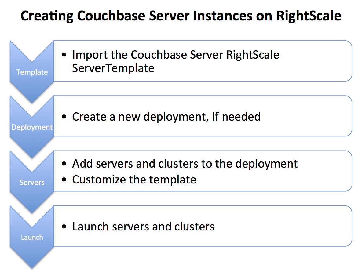
To set up Couchbase Server on RightScale, you need to import and customize a ServerTemplate. After the template is customized, you can launch server and cluster instances. The following figure illustrates the workflow:
The following procedures do not describe every parameter that you can modify when working with the RightScale ServerTemplates. If you need more information about a parameter, click the info button located near the parameter name.
To import the Couchbase Server RightScale ServerTemplate:
- From the RightScale menu bar, select Design > MultiCloud Marketplace > ServerTemplates.
- In the Keywords box on the left under Search, type couchbase, and then click Go.
-
In the search results list, click on the latest version of the Couchbase Server ServerTemplate.
The name of each Couchbase template in the list contains the Couchbase Server version number.
Click Import.
- Review each page of the end user license agreement, and then click Finish to accept the agreement.
To create a new deployment:
- From the RightScale menu bar, select Manage > Deployments > New.
- Enter a Nickname and Description for the new deployment.
- Click Save.
To add a server or cluster to a deployment:
- From the RightScale menu bar, select Manage > Deployments.
- Click the nickname of the deployment that you want to place the server or cluster in.
- From the deployment page menu bar, add the server or cluster:
- To add a server, click Add Server.
- To add a cluster, click Add Array.
- In the Add to Deployment window, select a cloud and click Continue.
-
On the Server Template page, select a template from the list.
If you have many server templates in your account, you can reduce the number of entries in the list by typing a keyword from the template name into the Server Template Name box under Filter Options.
Click Server Details.
-
On the Server Details page, choose settings for Hardware:
Server Name or Array Name—Enter a name for the new server or array.
Instance Type—The default is extra large. The template supports only large or extra large instances and requires a minimum of 4 cores.
EBS Optimized—Select the check box to enable EBS-optimized volumes for Provisioned IOPS.
-
Choose settings for Networking:
SSH Key—Choose an SSH key.
Security Groups—Choose one or more security groups.
-
If you are adding a cluster, click Array Details, and then choose settings for Autoscaling Policy and Array Type Details.
Under Autoscaling Policy, you can set the minimum and maximum number of active servers in the cluster by modifying the Min Count and Max Count parameters. If you want a specific number of servers, set both parameters to the same value.
Click Finish.
To customize the template for a server or a cluster:
- From the RightScale menu bar, select Manage > Deployments.
- Click the nickname of the deployment that the server or cluster is in.
- Click the nickname of the server or cluster.
- On the Server or Server Array page, click the Inputs tab, and then click edit.
-
Expand the BLOCK_DEVICE category and modify inputs as needed.
The BLOCK_DEVICE category contains input parameters that are specific to storage. Here’s a list of some advanced inputs that you might want to modify:
- I/O Operations per Second—Number of input/output operations per second (IOPS) that the volume can support
- Volume Type—Type of storage device
-
Expand the DB_COUCHBASE category and modify inputs as needed.
The DB_COUCHBASE category contains input parameters that are specific to Couchbase Server. In general, the default values are suitable for one server. If you want to create a cluster, you need to modify the input parameter values. Here’s a list of the advanced inputs that you can modify:
Bucket Name—Name of the bucket. The default bucket name is
default.Bucket Password—Password for the bucket.
Bucket RAM Quota—RAM quota for the bucket in MB.
Bucket Replica Count—Bucket replica count.
Cluster REST/Web Password—Password for the administrator account. The default is
password.Cluster REST/Web Username—Administrator account user name for access to the cluster via the REST or web interface. The default is
Administrator.Cluster Tag—Tag for nodes in the cluster that are automatically joined.
Couchbase Server Edition—The edition of Couchbase Server. The default is
enterprise.Rebalance Count—The number of servers to launch before doing a rebalance. Set this value to the total number of target servers you plan to have in the cluster. If you set the value to 0, Couchbase Server does a rebalance after each server joins the cluster.
Click Save.
- If you are ready to launch the server or cluster right now, click Launch.
To launch servers or clusters:
- From the RightScale menu bar, select Manage > Deployments.
- Click the nickname of the deployment that the server or cluster is in.
- Click the nickname of the server or cluster.
- On the Server or Server Array page, click Launch.
To log in to the Couchbase Web Console:
You can log in to the Couchbase Web Console by using your web browser to connect to the public IP address on port 8091. The general format is http://<server:port>. For example: if the public IP address is 192.236.176.4, enter http://192.236.176.4:8091/ in the web browser location bar.
Deployment strategies
Here are a number of deployment strategies that you may want to use. Smart clients are the preferred deployment option if your language and development environment supports a smart client library. If not, use the client-side Moxi configuration for the best performance and functionality.
Using a smart (vBucket aware) client
When using a smart client, the client library provides an interface to the cluster and performs server selection directly via the vBucket mechanism. The clients communicate with the cluster using a custom Couchbase protocol. This allows the clients to share the vBucket map, locate the node containing the required vBucket, and read and write information from there.
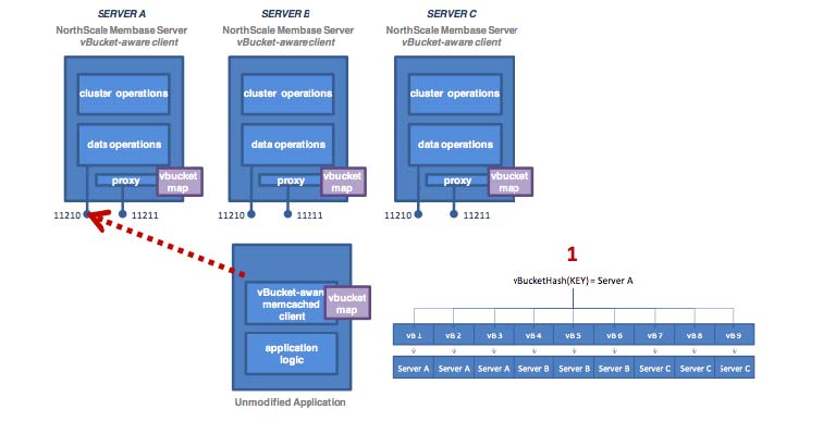
In releases prior to Couchbase Server 2.5, a developer, via a client library of their choice, randomly selects a host from which to request an initial topology configuration. Any future changes to the cluster map following the initial bootstrap are based on the NOT_MY_VBUCKET response from the server. This connection is made to port 8091 and is based on an HTTP connection.
Starting with Couchbase Server 2.5, client libraries query a cluster for initial topology configuration for a bucket from one of the nodes in the cluster. This is similar to prior releases. However, this information is transmitted via the memcached protocol on port 11210 (rather than via persistent HTTP connections to port 8091). This significantly improves connection scaling capabilities.
Optimized connection management is backward compatible. Old client libraries can connect to Couchbase Server 2.5, and updated client libraries can connect to Couchbase Server 2.5 and earlier.
Note
This change is only applicable to Couchbase type buckets (not memcached buckets).
See also vBuckets for an in-depth description.
Client-side (standalone) proxy
If a smart client is not available for your chosen platform, you can deploy a
standalone proxy. This provides the same functionality as the smart client while
presenting a memcached compatible interface layer locally. A standalone proxy
deployed on a client may also be able to provide valuable services, such as
connection pooling. The diagram below shows the flow with a standalone proxy
installed on the application server.
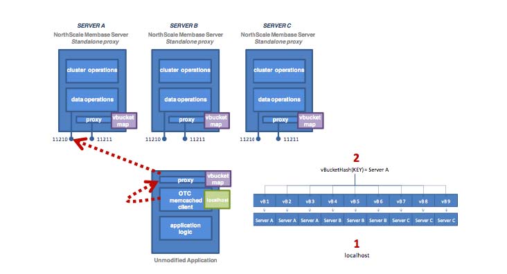
We configured the memcached client to have just one server in its server list
(localhost), so all operations are forwarded to localhost:11211 — a port
serviced by the proxy. The proxy hashes the document ID to a vBucket, looks up
the host server in the vBucket table, and then sends the operation to the
appropriate Couchbase Server on port 11210.
Note
For the corresponding Moxi product, please use the Moxi 1.8 series. See Moxi 1.8 Manual.
Using server-side (Couchbase embedded) proxy
Warning
We do not recommend server-side proxy configuration for production use. You should use either a smart client or the client-side proxy configuration unless your platform and environment do not support that deployment type.
The server-side (embedded) proxy exists within Couchbase Server using port 11211. It supports the memcached protocol and allows an existing application to communicate with Couchbase Cluster without installing another piece of proxy software. The downside to this approach is performance.
In this deployment option versus a typical memcached deployment, in a worse-case scenario, server mapping will happen twice (e.g. using Ketama hashing to a server list on the client, then using vBucket hashing and server mapping on the proxy) with an additional round trip network hop introduced.
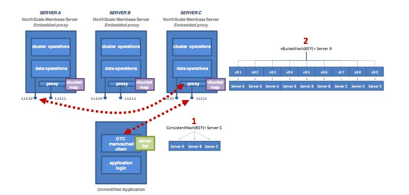
Note
For the corresponding Moxi product, please use the Moxi 1.8 series. See Moxi 1.8 Manual.
Couchbase Web Console
The Couchbase Web Console is the main tool for managing your Couchbase installation. The Web Console provides the following tabs:
-
Cluster Overview: a quick guide to the status of your Couchbase cluster.For more information, read Viewing Cluster Summary.
-
Data Buckets: view and update data bucket settings. You can create new buckets, edit existing settings, and see detailed statistics on the bucket.See Viewing Data Buckets.
-
Server Nodes: shows your active nodes, their configuration and activity. Under this tab you can also fail over nodes and remove them from your cluster, view server-specific performance, and monitor cluster statistics.Read Viewing Server Nodes.
-
Views: is were you can create and manage your views functions for indexing and querying data. Here you can also preview results from views.See Using the Views Editor for the views editor in Web Console. For more information on views in general, see Views and Indexes.
-
Documents: you can be create and edit documents under this tab. This enables you to view and modify documents that have been stored in a data bucket and can be useful when you work with views. -
Log: displays errors and problems.See Log for more information.
-
Settings: under this tab you can configure the console and cluster settings.See Settings for more information.
In addition to these sections of the Couchbase Web Console, there are additional systems within the web console, including:
-
Update NotificationsUpdate notifications indicates when there is an update available for the installed Couchbase Server. See Updating Notifications for more information on this feature.
-
Warnings and AlertsWarnings and alerts in Web Console will notify you when there is an issue that needs to be addressed within your cluster. The warnings and alerts can be configured through Settings.
For more information on the warnings and alerts, see Warnings and Alerts.
Viewing cluster summary
Cluster Overview is the home page for the Couchbase Web Console. The page
provides an overview of your cluster health, including RAM and disk usage and
activity. The page is divided into several sections: Cluster, Buckets, and Servers.
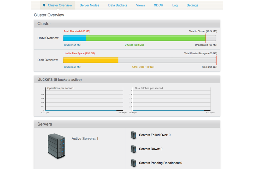
Viewing cluster overview
The Cluster section provides information on the RAM and disk usage information for your cluster.
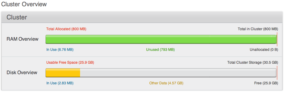
For the RAM information you are provided with a graphical representation of your RAM situation, including:
-
Total in ClusterTotal RAM configured within the cluster. This is the total amount of memory configured for all the servers within the cluster.
-
Total AllocatedThe amount of RAM allocated to data buckets within your cluster.
-
UnallocatedThe amount of RAM not allocated to data buckets within your cluster.
-
In UseThe amount of memory across all buckets that is actually in use (i.e. data is actively being stored).
-
UnusedThe amount of memory that is unused (available) for storing data.
The Disk Overview section provides similar summary information for disk
storage space across your cluster.
-
Total Cluster StorageTotal amount of disk storage available across your entire cluster for storing data.
-
Usable Free SpaceThe amount of usable space for storing information on disk. This figure shows the amount of space available on the configured path after non-Couchbase files have been taken into account.
-
Other DataThe quantity of disk space in use by data other than Couchbase information.
-
In UseThe amount of disk space being used to actively store information on disk.
-
FreeThe free space available for storing objects on disk.
Viewing buckets
The Buckets section provides two graphs showing the Operations per second
and Disk fetches per second.
The Operations per second provides information on the level of activity on the
cluster in terms of storing or retrieving objects from the data store.
The Disk fetches per second indicates how frequently Couchbase is having to go
to disk to retrieve information instead of using the information stored in RAM.
Viewing servers
The Servers section indicates overall server information for the cluster:
Active Serversis the number of active servers within the current cluster configuration.Servers Failed Overis the number of servers that have failed over due to an issue that should be investigated.Servers Downshows the number of servers that are down and not-contactable.Servers Pending Rebalanceshows the number of servers that are currently waiting to be rebalanced after joining a cluster or being reactivated after failover.
Viewing server nodes
In addition to monitoring buckets over all the nodes within the cluster, Couchbase Server also includes support for monitoring the statistics for an individual node.
The Server Nodes monitoring overview shows summary data for the Swap Usage, RAM Usage, CPU Usage and Active Items across all the nodes in your cluster.
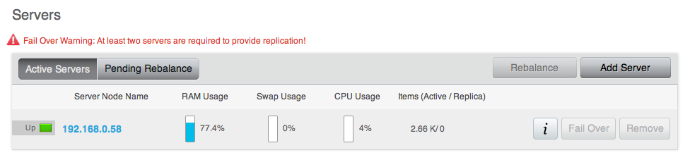
Clicking the triangle next to a server displays server node specific information, including the IP address, OS, Couchbase version and Memory and Disk allocation information.
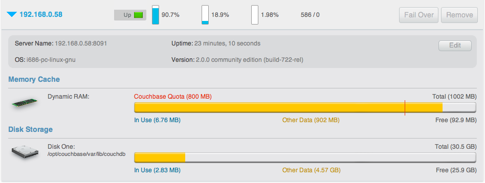
The detail display shows the following information:
-
Node information
The node information provides detail node configuration data:
-
Server NameThe server IP address and port number used to communicated with this sever.
-
UptimeThe uptime of the Couchbase Server process. This displays how long Couchbase Server has been running as a node, not the uptime for the server.
-
OSThe operating system identifier, showing the platform, environment, operating system and operating system derivative.
-
VersionThe version number of the Couchbase Server installed and running on this node.
-
-
Memory cache
The Memory Cache section shows you the information about memory usage, both for Couchbase Server and for the server as a whole. You can use this to compare RAM usage within Couchbase Server to the overall available RAM. The specific details tracked are:
-
Couchbase Quota
Shows the amount of RAM in the server allocated specifically to Couchbase Server.
-
In Use
Shows the amount of RAM currently in use by stored data by Couchbase Server.
-
Other Data
Shows the RAM used by other processes on the server.
-
Free
Shows the amount of free RAM out of the total RAM available on the server.
-
Total
Shows the total amount of free RAM on the server available for all processes.
-
-
Disk Storage
This section displays the amount of disk storage available and configured for Couchbase. Information will be displayed for each configured disk.
-
In Use
Shows the amount of disk space currently used to stored data for Couchbase Server.
-
Other Data
Shows the disk space used by other files on the configured device, not controlled by Couchbase Server.
-
Free
Shows the amount of free disk storage on the server out of the total disk space available.
-
Total
Shows the total disk size for the configured storage device.
-
Selecting a server from the list shows the server-specific version of the Bucket Monitoring overview, showing server-specific performance information.
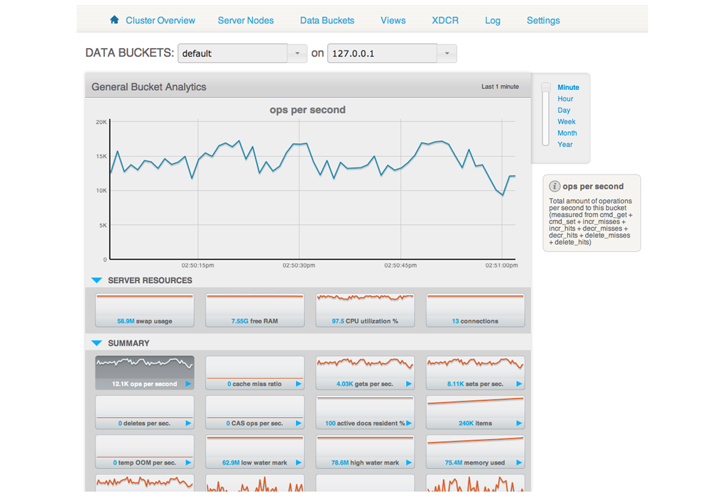
The graphs specific to the server are:
-
swap usage
Amount of swap space in use on this server.
-
free RAM
Amount of RAM available on this server.
-
CPU utilization
Percentage of CPU utilized across all cores on the selected server.
-
connection count
Number of connections to this server of all types for client, proxy, TAP requests and internal statistics.
By clicking on the blue triangle against an individual statistic within the server monitoring display, you can optionally select to view the information for a specific bucket-statistic on an individual server, instead of across the entire cluster.
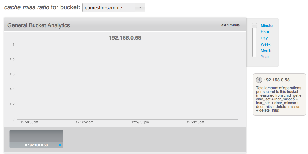
For more information on the data bucket statistics, see Viewing Data Buckets.
Understanding server states
Couchbase Server nodes can be in a number of different states depending on their current activity and availability. The displayed states are:
-
Up
Host is up, replicating data between nodes and servicing requests from clients.
-
Down
Host is down, not replicating data between nodes and not servicing requests from clients.
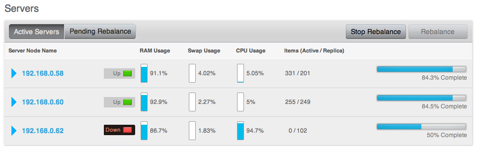
-
Pend
Host is up and currently filling RAM with data, but is not servicing requests from clients. Client access will be supported once the RAM has been pre-filled with information.
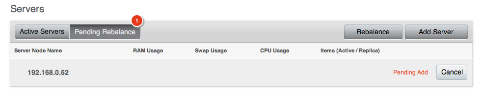
You can monitor the current server status using both the Manage: Server Nodes
and Monitor: Server Nodes screens within the Web Console.
Viewing data buckets
Couchbase Server provides a range of statistics and settings through the Data
Buckets and Server Nodes. These show overview and detailed information so
that administrators can better understand the current state of individual nodes
and the cluster as a whole.
The Data Buckets page displays a list of all the configured buckets on your
system (of both Couchbase and memcached types). The page provides a quick
overview of your cluster health from the perspective of the configured buckets,
rather than whole cluster or individual servers.
The information is shown in the form of a table, as seen in the figure below.
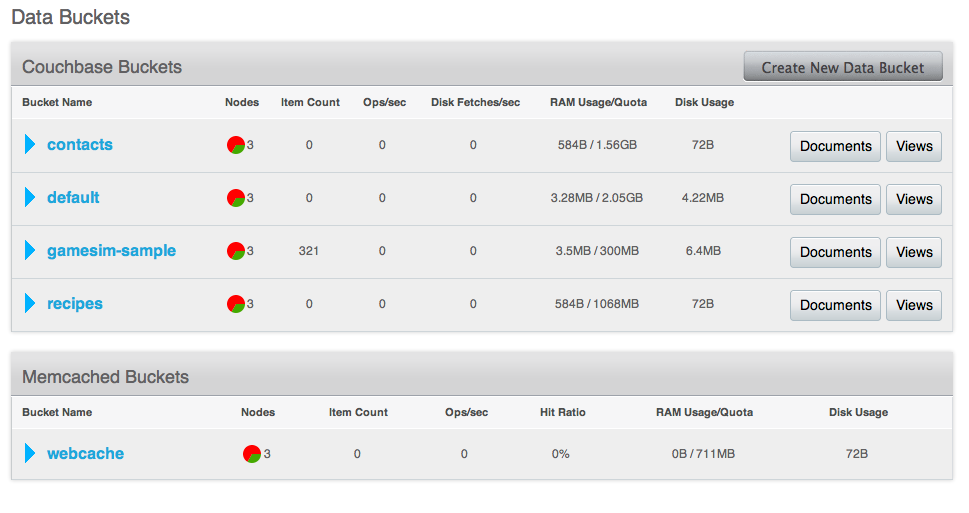
The list of buckets are separated by the bucket type. For each bucket, the following information is provided in each column:
Bucket nameis the given name for the bucket. Clicking on the bucket name takes you to the individual bucket statistics page. For more information, see Individual Bucket Monitoring.RAM Usage/Quotashows the amount of RAM used (for active objects) against the configure bucket size.Disk Usageshows the amount of disk space in use for active object data storage.Item Countindicates the number of objects stored in the bucket.Ops/secshows the number of operations per second for this data bucket.Disk Fetches/secshows the number of operations required to fetch items from disk.Clicking the
Bucket Nameopens the basic bucket information summary. For more information, see Bucket Information.Clicking the
Documentsbutton will take you to a list of objects identified as parseable documents. See Using the Document Editor for more information.The
Viewsbutton allows you to create and manage views on your stored objects. For more information, see Using the Views Editor.
To create a new data bucket, click the Create New Data Bucket. See Creating
and Editing Data Buckets
for details on creating new data buckets.
Creating and editing data buckets
When creating a new data bucket, or editing an existing one, you will be presented with the bucket configuration screen. From here you can set the memory size, access control and other settings, depending on whether you are editing or creating a new bucket, and the bucket type.
Creating a new bucket
You can create a new bucket in Couchbase Web Console under the Data Buckets tab.
-
Click Data Buckets | Create New Data Bucket. You see the
Create Bucketpanel, as follows: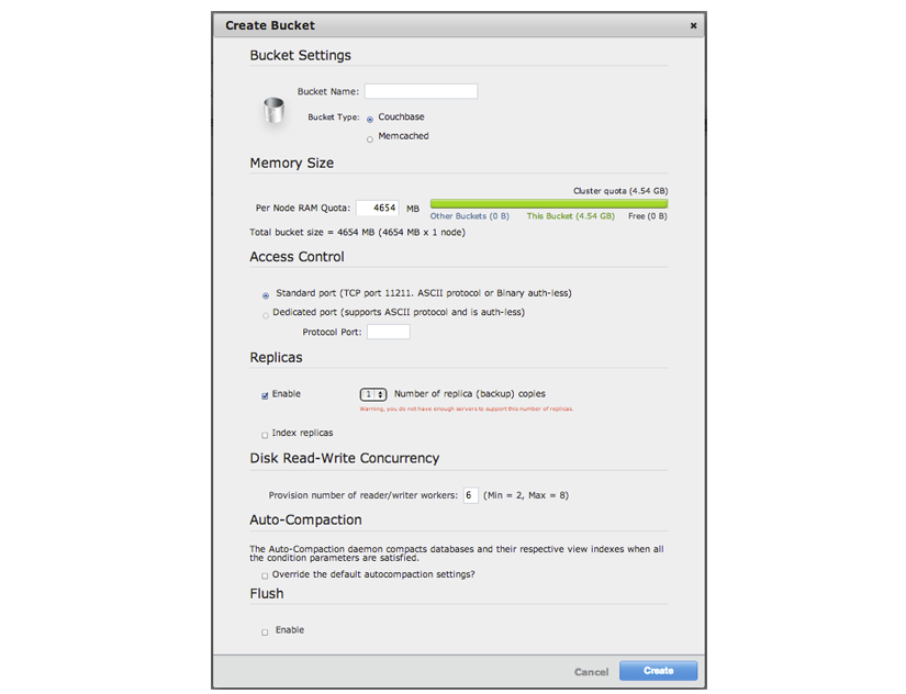
Select a name for the new bucket. The bucket name can only contain characters in range A-Z, a-z, 0-9 as well as underscore, period, dash and percent symbols.
Best Practice: Default Bucket Only for Testing
Create a named bucket specifically for your application. Any default bucket you initially set up with Couchbase Server should not be used for storing live application data. The default bucket you create when you first install Couchbase Server should be used only for testing.
-
Select a Bucket Type, either
MemcachedorCouchbase. See Data Storage for more information. The options that appear in this panel will differ based on your a bucket type you select.For
Couchbasebucket type:-
Memory Size
The amount of available RAM on this server which should be allocated to the bucket. Note that the allocation is the amount of memory that will be allocated for this bucket on each node, not the total size of the bucket across all nodes.
-
Replicas
For Couchbase buckets you can enable data replication so that the data is copied to other nodes in a cluster. You can configure up to three replicas per bucket. If you set this to one, you need to have a minimum of two nodes in your cluster and so forth. If a node in a cluster fails, after you perform failover, the replicated data will be made available on a functioning node. This provides continuous cluster operations in spite of machine failure. For more information, see Failver nodes.
You can disable replication by deselecting the
Enablecheckbox.You can disable replication by setting the number of replica copies to zero (0).
To configure replicas, Select a number in
Number of replica (backup) copiesdrop-down list.To enable replica indexes, Select the
Index replicascheckbox. Couchbase Server can also create replicas of indexes. This ensures that indexes do not need to be rebuilt in the event of a node failure. This will increase network load as the index information is replicated along with the data. -
Disk Read-Write Concurrency
Multiple readers and writers are supported to persist data onto disk. For earlier versions of Couchbase Server, each server instance had only single disk reader and writer threads. By default this is set to three total threads per data bucket, with two reader threads and one writer thread for the bucket.
For now, leave this setting at the default. In the future, when you create new data buckets you can update this setting. For general information about disk storage, see Disk Storage. For information on multi- readers and writers, see Using Multi- Readers and Writers.
-
Flush
To enable the operation for a bucket, click the
Enablecheckbox. Enable or disable support for the Flush command, which deletes all the data in an a bucket. The default is for the flush operation to be disabled.
For
Memcachedbucket type:-
Memory Size
The bucket is configured with a per-node amount of memory. Total bucket memory will change as nodes are added/removed.
For more information, see RAM Sizing.
Warning
Changing the size of a memcached bucket will erase all the data in the bucket and recreate it, resulting in loss of all stored data for existing buckets.
-
Auto-Compaction
Both data and index information stored on disk can become fragmented. Compaction rebuilds the stored data on index to reduce the fragmentation of the data. For more information on database and view compaction, see Database and View Compaction.
You can opt to override the default auto compaction settings for this individual bucket. Default settings are configured through the
Settingsmenu. For more information on setting the default autocompaction parameters, see Enabling Auto-Compaction. If you override the default autocompaction settings, you can configure the same parameters, but the limits will affect only this bucket.
For either bucket type provide these two settings in the Create Bucket panel:
-
Access ControlThe access control configures the port clients use to communicate with the data bucket, and whether the bucket requires a password.
To use the TCP standard port (11211), the first bucket you create can use this port without requiring SASL authentication. For each subsequent bucket, you must specify the password to be used for SASL authentication, and client communication must be made using the binary protocol.
To use a dedicated port, select the dedicate port radio button and enter the port number you want to use. Using a dedicated port supports both the text and binary client protocols, and does not require authentication.
Note: When defining a port on a bucket, the server automatically starts up a copy of Moxi on the servers, and exposes it on that port. This supports the ASCII memcached protocol. However, Couchbase strongly recommend against using Moxi in this way. If needed, a client-side Moxi should be installed on the application servers and have it connect to this bucket (whether it is “port” or “password” doesn’t matter).
When defining a password on a bucket, it requires a client that supports the binary memcached protocol with SASL (all Couchbase client libraries and client-side Moxi provide this support). Defining a password on a bucket is the recommended approach.
-
Flush
Enable or disable support for the Flush command, which deletes all the data in an a bucket. The default is for the flush operation to be disabled. To enable the operation for a bucket, click the
Enablecheckbox.
-
-
-
Click Create.
Creates the new bucket with bucket configuration.
Editing Couchbase buckets
You can edit a number of settings for an existing Couchbase bucket in Couchbase Web Console:
Access Control, including the standard port/password or custom port settings.Memory Sizecan be modified providing you have unallocated space within your Cluster configuration. You can reduce the amount of memory allocated to a bucket if that space is not already in use.Auto-Compactionsettings, including enabling the override of the default auto-compaction settings, and bucket-specific auto-compaction.Flushsupport. You can enable or disable support for the Flush command.
The bucket name cannot be modified. To delete the configured bucket entirely,
click the Delete button.
Editing Memcached buckets
For Memcached buckets, you can modify the following settings when editing an existing bucket:
Access Control, including the standard port/password or custom port settings.Memory Sizecan be modified providing you have unallocated RAM quota within your Cluster configuration. You can reduce the amount of memory allocated to a bucket if that space is not already in use.
You can delete the bucket entirely by clicking the Delete button.
You can empty a Memcached bucket of all the cached information that it stores by
using the Flush button.
Warning
Using the Flush button removes all the objects stored in the Memcached bucket. Using this button on active Memcached buckets may delete important information.
Bucket information
You can obtain basic information about the status of your data buckets by
clicking on the drop-down next to the bucket name under the Data Buckets page.
The bucket information shows memory size, access, and replica information for
the bucket, as shown in the figure below.
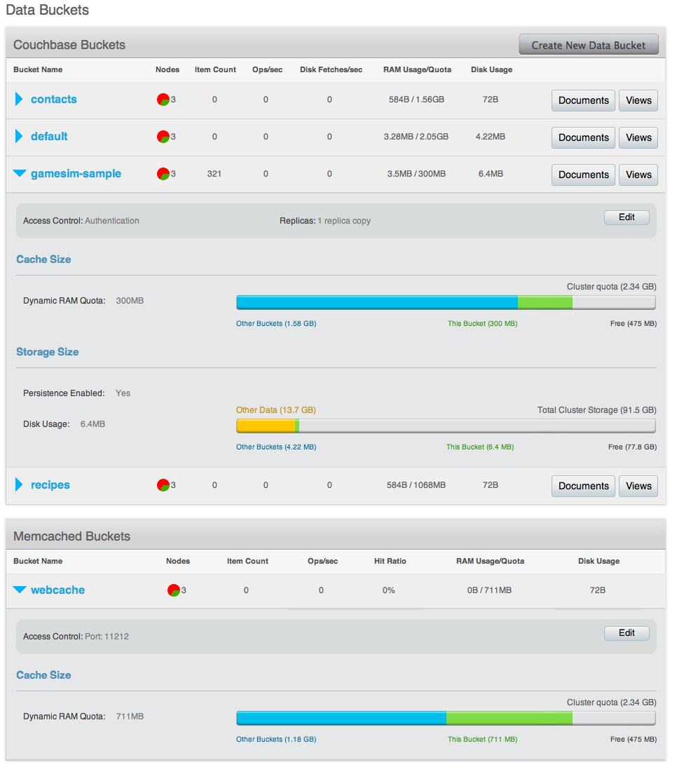
You can edit the bucket information by clicking the Edit button within the
bucket information display.
Viewing bucket and cluster statistics
Within the Data Bucket monitor display, information is shown by default for
the entire Couchbase Server cluster. The information is aggregated from all the
server nodes within the configured cluster for the selected bucket.
The following functionality is available through this display, and is common to all the graphs and statistics display within the web console.
-
Bucket SelectionThe
Data Bucketsselection list allows you to select which of the buckets configured on your cluster is to be used as the basis for the graph display. The statistics shown are aggregated over the whole cluster for the selected bucket. -
Server SelectionThe
Server Selectionoption enables you to limit the display to an individual server or entire cluster. You can select an individual node, which displays the Viewing Server Nodes for that node. SelectingAll Server Nodesshows the Viewing Data Buckets page. -
Interval SelectionThe
Interval Selectionat the top of the main graph changes interval display for all graphs displayed on the page. For example, selectingMinuteshows information for the last minute, continuously updating.
Note
As the selected interval increases, the amount of statistical data displayed will depend on how long your cluster has been running.
-
Statistic SelectionAll of the graphs within the display update simultaneously. Clicking on any of the smaller graphs will promote that graph to be displayed as the main graph for the page.
-
Individual Server SelectionClicking the blue triangle next to any of the smaller statistics graphs enables you to show the selected statistic individual for each server within the cluster, instead of aggregating the information for the entire cluster.
Individual bucket monitoring
Bucket monitoring within the Couchbase Web Console has been updated to show additional detailed information. The following statistic groups are available for Couchbase bucket types.
-
Summary
The summary section provides a quick overview of the cluster activity. For more information, see Bucket Monitoring — Summary Statistics.
-
vBucket Resources
This section provides detailed information on the vBucket resources across the cluster, including the active, replica and pending operations. For more information, see Monitoring vBucket Resources.
-
Disk Queues
Disk queues show the activity on the backend disk storage used for persistence within a data bucket. The information displayed shows the active, replica and pending activity. For more information, see Monitoring Disk Queues.
-
TAP Queues
The TAP queues section provides information on the activity within the TAP queues across replication, rebalancing and client activity. For more information, see Monitoring TAP Queues.
-
XDCR Destination
The XDCR Destination section show you statistical information about the Cross Datacenter Replication (XDCR), if XDCR has been configured. For more information on XDCR, see Cross Datacenter Replication (XDCR). For more information on the available statistics, see Monitoring Outgoing XDCR.
-
View Stats
The View Stats section allows you to monitor the statistics for each production view configured within the bucket or system. For more information on the available statistics, see Monitoring View Statistics.
-
Top Keys
This shows a list of the top 10 most actively used keys within the selected data bucket.
For Memcached bucket types, the Memcached statistic summary is provided. See Bucket Memcached Buckets.
Bucket monitoring — summary statistics
The summary section is designed to provide a quick overview of the cluster activity. Each graph (or selected graph) shows information based on the currently selected bucket.
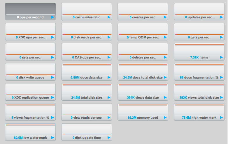
The following graph types are available:
-
ops per secondThe total number of operations per second on this bucket.
-
cache miss ratioRatio of reads per second to this bucket which required a read from disk rather than RAM.
-
creates per secondNumber of new items created in this bucket per second.
-
updates per secondNumber of existing items updated in this bucket per second.
-
XDCR ops per secNumber of XDCR related operations per second for this bucket.
-
disk reads per secNumber of reads per second from disk for this bucket.
-
temp OOM per secNumber of temporary out of memory conditions per second.
-
gets per secondNumber of get operations per second.
-
sets per secondNumber of set operations per second.
-
deletes per secondNumber of delete operations per second.
-
itemsNumber of items (documents) stored in the bucket.
-
disk write queueSize of the disk write queue.
-
docs data sizeSize of the stored document data.
-
docs total disk sizeSize of the persisted stored document data on disk.
-
doc fragmentation %Document fragmentation of persisted data as stored on disk.
-
XDC replication queueSize of the XDCR replication queue.
-
total disk sizeTotal size of the information for this bucket as stored on disk, including persisted and view index data.
-
views data sizeSize of the view data information.
-
views total disk sizeSize of the view index information as stored on disk.
-
views fragmentation %Percentage of fragmentation for a given view index.
-
view reads per secondNumber of view reads per second.
-
memory usedAmount of memory used for storing the information in this bucket.
-
high water markHigh water mark for this bucket (based on the configured bucket RAM quota).
-
low water markLow water mark for this bucket (based on the configured bucket RAM quota).
-
disk update timeTime required to update data on disk.
Monitoring vBucket resources
The vBucket statistics provide information for all vBucket types within the cluster across three different states. Within the statistic display the table of statistics is organized in four columns, showing the Active, Replica and Pending states for each individual statistic. The final column provides the total value for each statistic.

The Active column displays the information for vBuckets within the Active state. The Replica column displays the statistics for vBuckets within the Replica state (i.e. currently being replicated). The Pending columns shows statistics for vBuckets in the Pending state, i.e. while data is being exchanged during rebalancing.
These states are shared across all the following statistics. For example, the
graph new items per sec within the Active state column displays the number
of new items per second created within the vBuckets that are in the active
state.
The individual statistics, one for each state, shown are:
-
vBucketsThe number of vBuckets within the specified state.
-
itemsNumber of items within the vBucket of the specified state.
-
resident %Percentage of items within the vBuckets of the specified state that are resident (in RAM).
-
new items per sec.Number of new items created in vBuckets within the specified state. Note that new items per second is not valid for the Pending state.
-
ejections per secondNumber of items ejected per second within the vBuckets of the specified state.
-
user data in RAMSize of user data within vBuckets of the specified state that are resident in RAM.
-
metadata in RAMSize of item metadata within the vBuckets of the specified state that are resident in RAM.
Monitoring disk queues
The Disk Queues statistics section displays the information for data being placed into the disk queue. Disk queues are used within Couchbase Server to store the information written to RAM on disk for persistence. Information is displayed for each of the disk queue states, Active, Replica and Pending.
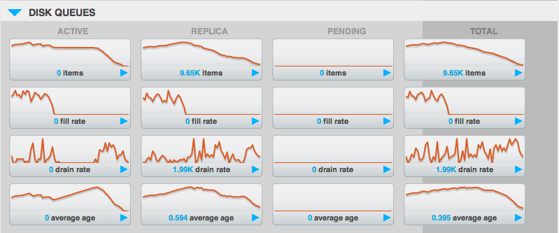
The Active column displays the information for the Disk Queues within the Active state. The Replica column displays the statistics for the Disk Queues within the Replica state (i.e. currently being replicated). The Pending columns shows statistics for the disk Queues in the Pending state, i.e. while data is being exchanged during rebalancing.
These states are shared across all the following statistics. For example, the
graph fill rate within the Replica state column displays the number of items
being put into the replica disk queue for the selected bucket.
The displayed statistics are:
-
itemsThe number of items waiting to be written to disk for this bucket for this state.
-
fill rateThe number of items per second being added to the disk queue for the corresponding state.
-
drain rateNumber of items actually written to disk from the disk queue for the corresponding state.
-
average ageThe average age of items (in seconds) within the disk queue for the specified state.
Monitoring TAP queues
The TAP queues statistics are designed to show information about the TAP queue activity, both internally, between cluster nodes and clients. The statistics information is therefore organized as a table with columns showing the statistics for TAP queues used for replication, rebalancing and clients.
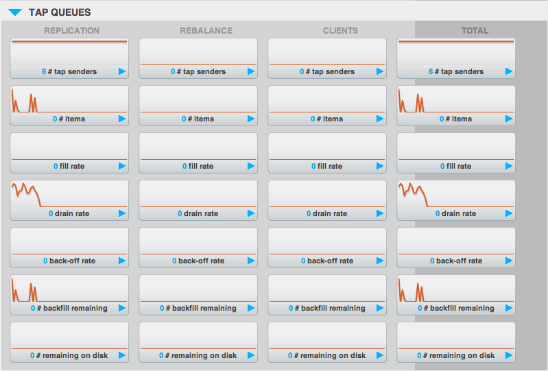
The statistics in this section are detailed below:
-
TAP sendersNumber of TAP queues in this bucket for internal (replica), rebalancing or client connections.
-
itemsNumber of items in the corresponding TAP queue for this bucket.
-
drain rateNumber of items per second being sent over the corresponding TAP queue connections to this bucket.
-
back-off rateNumber of back-offs per second sent when sending data through the corresponding TAP connection to this bucket.
-
backfill remainingNumber of items in the backfill queue for the corresponding TAP connection for this bucket.
-
remaining on diskNumber of items still on disk that need to be loaded in order to service the TAP connection to this bucket.
Memcached buckets
For Memcached buckets, Web Console displays a separate group of statistics:
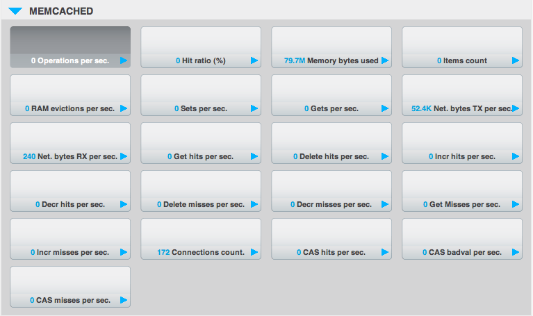
The Memcached statistics are:
-
Operations per sec.Total operations per second serviced by this bucket
-
Hit Ratio %Percentage of get requests served with data from this bucket
-
Memory bytes usedTotal amount of RAM used by this bucket
-
Items countNumber of items stored in this bucket
-
RAM evictions per sec.Number of items per second evicted from this bucket
-
Sets per sec.Number of set operations serviced by this bucket
-
Gets per sec.Number of get operations serviced by this bucket
-
Net. bytes TX per secNumber of bytes per second sent from this bucket
-
Net. bytes RX per sec.Number of bytes per second sent into this bucket
-
Get hits per sec.Number of get operations per second for data that this bucket contains
-
Delete hits per sec.Number of delete operations per second for data that this bucket contains
-
Incr hits per sec.Number of increment operations per second for data that this bucket contains
-
Decr hits per sec.Number of decrement operations per second for data that this bucket contains
-
Delete misses per sec.Number of delete operations per second for data that this bucket does not contain
-
Decr misses per sec.Number of decr operations per second for data that this bucket does not contain
-
Get Misses per sec.Number of get operations per second for data that this bucket does not contain
-
Incr misses per sec.Number of increment operations per second for data that this bucket does not contain
-
CAS hits per sec.Number of CAS operations per second for data that this bucket contains
-
CAS badval per sec.Number of CAS operations per second using an incorrect CAS ID for data that this bucket contains
-
CAS misses per sec.Number of CAS operations per second for data that this bucket does not contain
Monitoring outgoing XDCR
The Outgoing XDCR shows the XDCR operations that are supporting cross datacenter replication from the current cluster to a destination cluster. For more information on XDCR, see Cross Datacenter Replication (XDCR).
You can monitor the current status for all active replications in the Ongoing
Replications section under the XDCR tab:
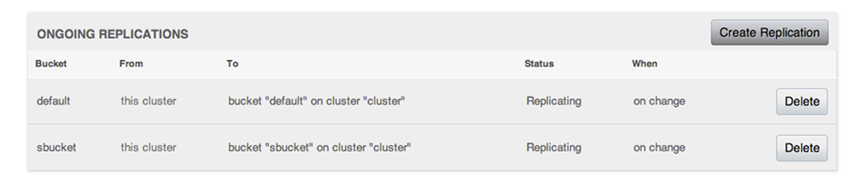
The Ongoing Replications section shows the following information:
| Column | Description |
|---|---|
| Bucket | The source bucket on the current cluster that is being replicated. |
| From | Source cluster name. |
| To | Destination cluster name. |
| Status | Current status of replications. |
| When | Indicates when replication occurs. |
The Status column indicates the current state of the replication
configuration. Possible include:
-
Starting Up
The replication process has just started, and the clusters are determining what data needs to be sent from the originating cluster to the destination cluster.
-
Replicating
The bucket is currently being replicated and changes to the data stored on the originating cluster are being sent to the destination cluster.
-
Failed
Replication to the destination cluster has failed. The destination cluster cannot be reached. The replication configuration may need to be deleted and recreated.
Under the Data Buckets tab you can click on a named Couchbase bucket and find
more statistics about replication for that bucket. Couchbase Web Console
displays statistics for the particular bucket; on this page you can find two
drop-down areas called in the Outgoing XDCR and Incoming XDCR Operations.
Both provides statistics about ongoing replication for the particular bucket.
Under the Outgoing XDCR panel if you have multiple replication streams you
will see statistics for each stream.
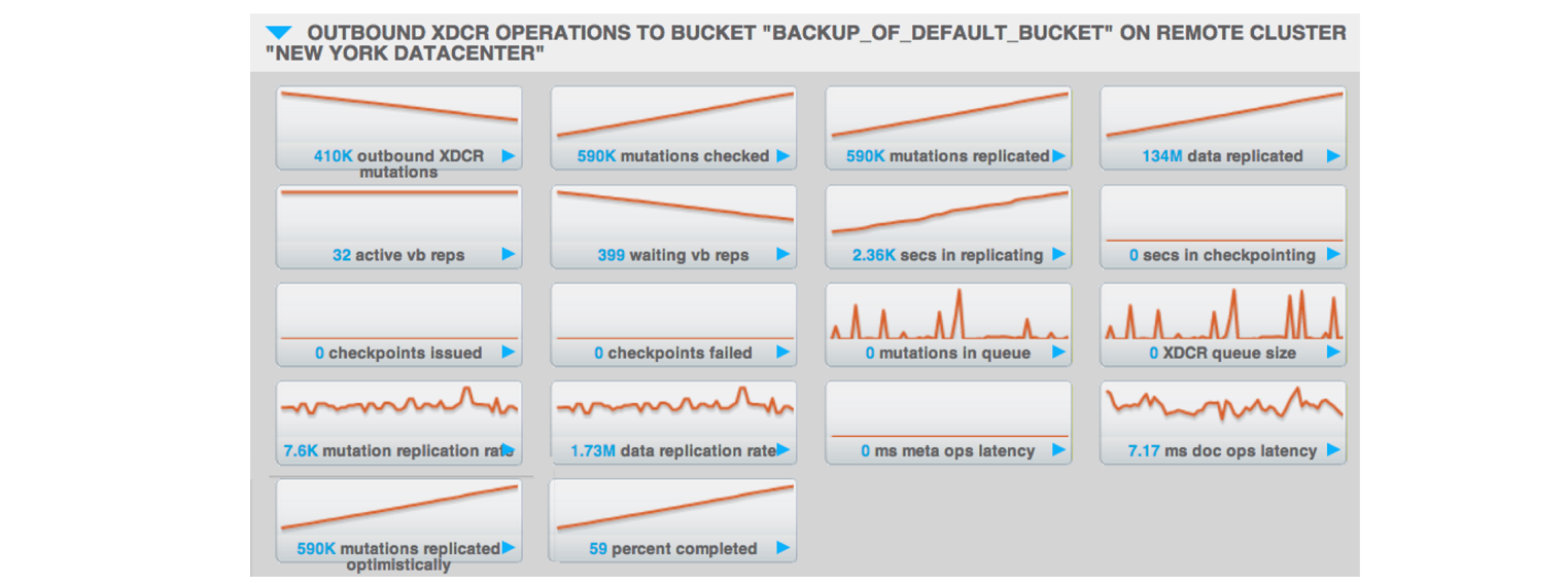
The statistics shown are:
-
outbound XDCR mutationNumber of changes in the queue waiting to be sent to the destination cluster.
-
mutations checkedNumber of document mutations checked on source cluster.
-
mutations replicatedNumber of document mutations replicated to the destination cluster.
-
data replicatedSize of data replicated in bytes.
-
active vb repsNumber of parallel, active vBucket replicators. Each vBucket has one replicator which can be active or waiting. By default you can only have 32 parallel active replicators at once per node. Once an active replicator finishes, it will pass a token to a waiting replicator.
-
waiting vb repsNumber of vBucket replicators that are waiting for a token to replicate.
-
secs in replicatingTotal seconds elapsed for data replication for all vBuckets in a cluster.
-
secs in checkpointingTime working in seconds including wait time for replication.
-
checkpoints issuedTotal number of checkpoints issued in replication queue. By default active vBucket replicators issue a checkpoint every 30 minutes to keep track of replication progress.
-
checkpoints failedNumber of checkpoints failed during replication. This can happen due to timeouts, due to network issues or if a destination cluster cannot persist quickly enough.
-
mutations in queueNumber of document mutations waiting in replication queue.
-
XDCR queue sizeAmount of memory used by mutations waiting in replication queue. In bytes.
-
mutation replication rateNumber of mutations replicated to destination cluster per second.
-
data replication rateBytes replicated to destination per second.
-
ms meta ops latencyWeighted average time for requesting document metadata. In milliseconds.
-
mutations replicated optimisticallyTotal number of mutations replicated with optimistic XDCR.
-
ms docs ops latencyWeighted average time for sending mutations to destination cluster. In milliseconds.
-
percent completedPercent of total mutations checked for metadata.
Be aware that if you use an earlier version of Couchbase Server, such as Couchbase Server 2.0, only the first three statistics appear and have the labels changes queue, documents checked, and documents replicated respectively. You can also get XDCR statistics using the Couchbase REST API. All of the statistics in Web Console are based on statistics via the REST API or values derived from them. For more information including a full list of available statistics, see Getting XDCR Stats via REST.
Monitoring incoming XDCR
The Incoming XDCR section shows the XDCR operations that are coming into to the current cluster from a remote cluster. For more information on XDCR, see Cross Datacenter Replication (XDCR).
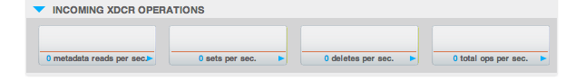
The statistics shown are:
-
metadata reads per sec.Number of documents XDCR scans for metadata per second. XDCR uses this information for conflict resolution. See, Behavior and Limitations.
-
sets per sec.Set operations per second for incoming XDCR data.
-
deletes per sec.Delete operations per second as a result of the incoming XDCR data stream.
-
total ops per sec.Total of all the operations per second.
Monitoring view statistics
The View statistics show information about individual design documents within the selected bucket. One block of stats will be shown for each production-level design document. For more information on Views, see Views and Indexes.
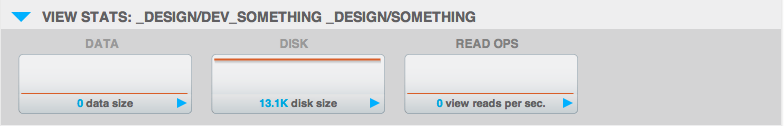
The statistics shown are:
-
data sizeSize of the data required for this design document.
-
disk sizeSize of the stored index as stored on disk.
-
view reads per sec.Number of read operations per second for this view.
Using the Views Editor
The Views Editor is available within the Couchbase Web Console. You can access
the View Editor either by clicking the Views for a given data bucket within
the Data Buckets display, or by selecting the Views page from the main
navigation panel.
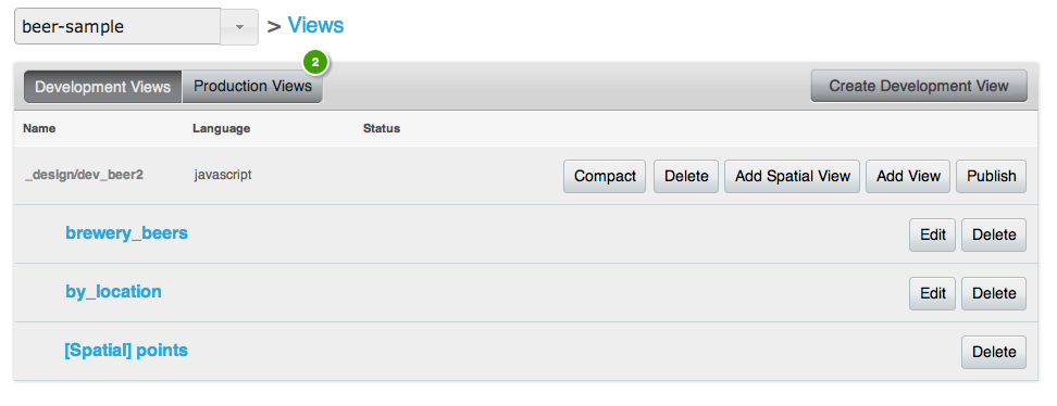
The individual elements of this interface are:
The pop-up, at the top-left, provides the selection of the data bucket where you are viewing or editing a view.
The
Create Development Viewenables you to create a new view either within the current design document, or within a new document. See Creating and Editing Views.You can switch between
Production ViewsandDevelopment Views. See Development and Production Views for more information.-
The final section provides a list of the design documents, and within each document, each defined view.
When viewing
Development Views, you can perform the following actions:Compactthe view index with an associated design document. This will compact the view index and recover space used to store the view index on disk.Deletea design document. This will delete all of the views defined within the design document.Add Spatial Viewcreates a new spatial view within the corresponding design document. See Creating and Editing Views.Add Viewcreates a new view within the corresponding design document. See Creating and Editing Views.Publishyour design document (and all of the defined views) as a production design document. See Publishing Views.-
For each individual view listed:
-
Edit, or clicking the view nameOpens the view editor for the current view name, see Creating and Editing Views.
-
DeleteDeletes an individual view.
-
When viewing
Production Viewsyou can perform the following operations on each design document:Compactthe view index with an associated design document. This will compact the view index and recover space used to store the view index on disk.Deletea design document. This will delete all of the views defined within the design document.Copy to Devcopies the view definition to the development area of the view editor. This enables you edit the view definition. Once you have finished making changes, using thePublishbutton will then overwrite the existing view definition.-
For each individual view:
- By clicking the view name, or the
Showbutton, execute and examine the results of a production view. See Getting View Results for more information.
- By clicking the view name, or the
Creating and editing views
You can create a new design document and/or view by clicking the Create
Development View button within the Views section of the Web Console. If you
are creating a new design document and view you will be prompted to supply both
the design document and view name. To create or edit your documents using the
REST API, see the Design Document REST API.
To create a new view as part of an existing design document, click the Add
View button against the corresponding design document.
Note
View names must be specified using one or more UTF-8 characters. You cannot have a blank view name. View names cannot have leading or trailing whitespace characters (space, tab, newline, or carriage-return).
If you create a new view, or have selected a Development view, you can create
and edit the map() and reduce() functions. Within a development view, the
results shown for the view are executed either over a small subset of the full
document set (which is quicker and places less load on the system), or the full
data set.
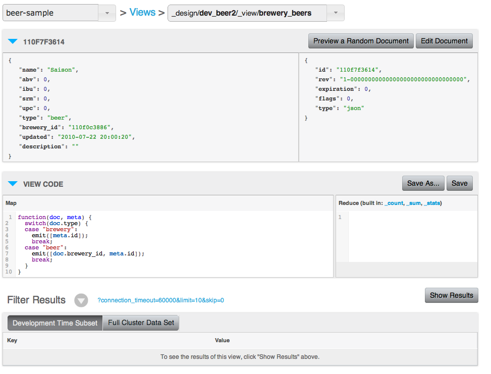
The top portion of the interface provides navigation between the available design documents and views.
The Sample Document section allows you to view a random document from the
database to help you write your view functions and so that you can compare the
document content with the generated view output. Clicking the Preview a Random
Document will randomly select a document from the database. Clicking Edit
Document will take you to the Views editor, see Using the Document
Editor
Note
Documents stored in the database that are identified as Non-JSON may be displayed as binary, or text-encoded binary, within the UI.
Document metadata is displayed in a separate box on the right hand side of the
associated document. This shows the metadata for the displayed document, as
supplied to the map() as the second argument to the function. For more
information on writing views and creating the map() and reduce() functions,
see Writing Views.
With the View Code section, you should enter the function that you want to use
for the map() and reduce() portions of the view. The map function is
required, the reduce function is optional. When creating a new view a basic
map() function will be provided. You can modify this function to output the
information in your view that you require.
Once you have edited your map() and reduce() functions, you must use the
Save button to save the view definition.
The design document will be validated before it is created or updated in the system. The validation checks for valid JavaScript and for the use of valid built-in reduce functions. Any validation failure is reported as an error.
You can also save the modified version of your view as a new view using the
Save As... button.
The lower section of the window will show you the list of documents that would
be generated by the view. You can use the Show Results to execute the view.
To execute a view and get a sample of the output generated by the view
operation, click the Show Results button. This will create the index and show
the view output within the table below. You can configure the different
parameters by clicking the arrow next to Filter Results. This shows the view
selection criteria, as seen in the figure below. For more information on
querying and selecting information from a view, see Querying
Views.
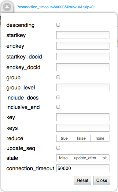
Clicking on the Filter Results query string will open a new window containing
the raw, JSON formatted, version of the View results. To access the view results
using the REST API, see the REST API, Querying views.
By default, Views during the development stage are executed only over a subset
of the full document set. This is indicated by the Development Time Subset
button. You can execute the view over the full document set by selecting Full
Cluster Data Set. Because this executes the view in real-time on the data set,
the time required to build the view may be considerable. Progress for building
the view is shown at the top of the window.
Note
If you have edited either the map() or reduce() portions of your view definition, you must save the definition. The Show Results button will
remain greyed out until the view definition has been saved.
You can also filter the results and the output using the built-in filter system. This filter provides similar options that are available to clients for filtering results.
For more information on the filter options, see Getting View Results.
Publishing views
Publishing a view moves the view definition from the Development view to a Production View. Production views cannot be edited. The act of publishing a view and moving the view from the development to the production view will overwrite a view the same name on the production side. To edit a Production view, you copy the view from production to development, edit the view definition, and then publish the updated version of the view back to the production side.
Getting view results
Once a view has been published to be a production view, you can examine and manipulate the results of the view from within the web console view interface. This makes it easy to study the output of a view without using a suitable client library to obtain the information.
To examine the output of a view, click icon next to the view name within the view list. This will present you with a view similar to that shown in the figure below.
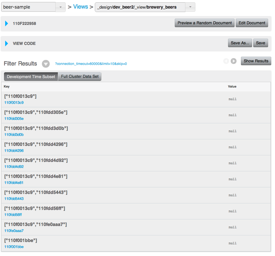
The top portion of the interface provides navigation between the available design documents and views.
The Sample Document section allows you to view a random document from the
database so that you can compare the document content with the generated view
output. Clicking the Preview a Random Document will randomly select a document
from the database. If you know the ID of a document that you want to examine,
enter the document ID in the box, and click the Lookup Id button to load the
specified document.
To examine the function that generate the view information, use the View Code
section of the display. This will show the configured map and reduce functions.
The lower portion of the window will show you the list of documents generated by
the view. You can use the Show Results to execute the view.
The Filter Results interface allows you to query and filter the view results
by selecting the sort order, key range, or document range, and view result
limits and offsets.
To specify the filter results, click on the pop-up triangle next to Filter
Results. You can delete existing filters, and add new filters using the
embedded selection windows. Click Show Results when you have finished
selecting filter values. The filter values you specify are identical to those
available when querying from a standard client library. For more information,
see Querying Views.
Note
Due to the nature of range queries, a special character may be added to query specifications when viewing document ranges. The character may not show up in all web browsers, and may instead appear instead as an invisible, but selectable, character. For more information on this character and usage, see Partial Selection and Key Ranges.
Using the Document Editor
The Document Viewer and Editor enables you to browse, view, and edit individual
documents stored in Couchbase Server buckets. To get to the Documents editor,
click on the Documents button within the Data Buckets view. This will open a
list of available documents. You are shown only a selection of the available
documents, rather than all documents. The maximum size of editable documents is 2.5 KB.
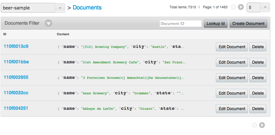
You can select a different Bucket by using the bucket selection popup on the
left. You can also page through the list of documents shown by using the
navigation arrows on the right. To jump to a specific document ID, enter the ID
in the box provided and click Lookup Id. To edit an existing document, click
the Edit Document button. To delete the document from the bucket, click
Delete.
To create a new document, click the Create Document button. This will open a
prompt to specify the document Id of the created document.
Once the document Id has been set, you will be presented with the document editor. The document editor will also be opened when you click on the document ID within the document list. To edit the contents of the document, use the textbox to modify the JSON of the stored document.
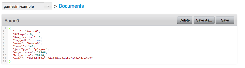
Within the document editor, you can click Delete to delete the current
document, Save As... will copy the currently displayed information and create
a new document with the document Id you specify. The Save will save the
current document and return you to the list of documents.
Log
The Log section of the website allows you to view the built-in event log for
Couchbase Server so that you can identify activity and errors within your
Couchbase cluster.
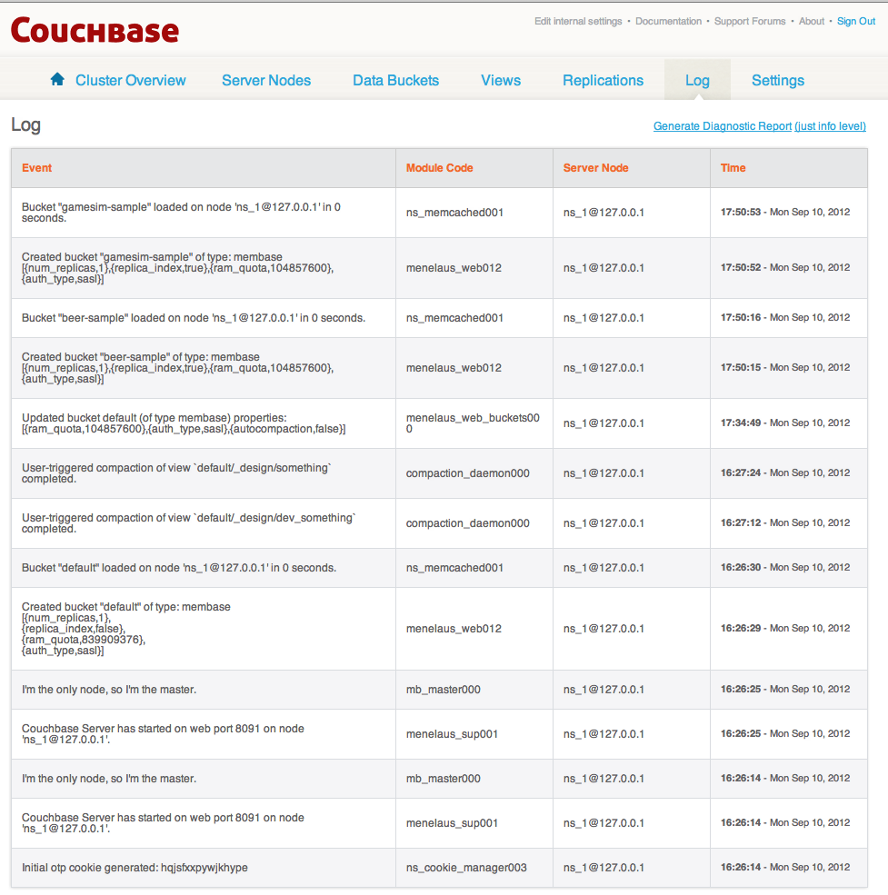
Settings
The Settings interface sets the global settings for your Couchbase Server
instance.
Cluster settings
Cluster settings show the available RAM on your cluster and the per server RAM quota. The Per Server RAM Quota is adjustable. In addition, if you have the Enterprise Edition, a Couchbase Server self-signed SSL certification is provided to set up secure communication in an XDCR environment. The SSL certificate can be regenerated. See XDCR data encryption for more information.
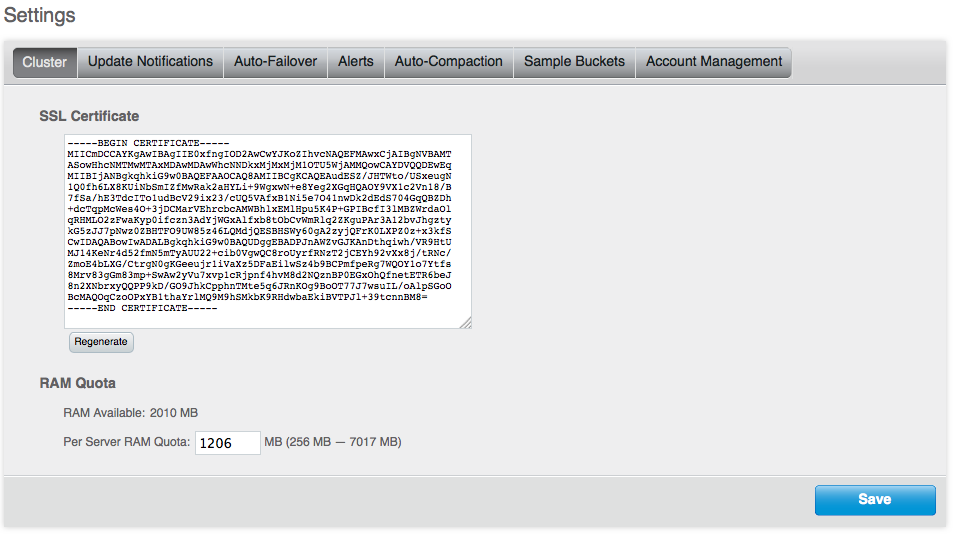
Update notification settings
You can enable or disable Update Notifications by checking the Enable software
update notifications checkbox within the Update Notifications screen. Once
you have changed the option, you must click Save to record the change.
If update notifications are disabled then the Update Notifications screen will only notify you of your currently installed version, and no alert will be provided.
For more information on how Update Notifications work, see Updating Notifications.
Enabling auto-failover settings
The Auto-Failover settings enable auto-failover, and the timeout before the auto-failover process is started when a cluster node failure is detected.
To enable Auto-Failover, check the Enable auto-failover checkbox. To set the
delay, in seconds, before auto-failover is started, enter the number of seconds
it the Timeout box. The default timeout is 120 seconds. For more information on Auto-Failover, see Using Automatic Failover.
Enabling alerts
You can enable email alerts to be raised when a significant error occurs on your Couchbase Server cluster. The email alert system works by sending email directly to a configured SMTP server. Each alert email is sent to the list of configured email recipients.
The available settings are:
-
Enable email alertsIf checked, email alerts will be raised on the specific error enabled within the
Available Alertssection of the configuration. -
HostThe hostname for the SMTP server that will be used to send the email.
-
PortThe TCP/IP port to be used to communicate with the SMTP server. The default is the standard SMTP port 25.
-
UsernameFor email servers that require a username and password to send email, the username for authentication.
-
PasswordFor email servers that require a username and password to send email, the password for authentication.
-
Require TLSEnable Transport Layer Security (TLS) when sending the email through the designated server.
-
Sender emailThe email address from which the email will be identified as being sent from. This email address should be one that is valid as a sender address for the SMTP server that you specify.
-
RecipientsA list of the recipients of each alert message. You can specify more than one recipient by separating each address by a space, comma or semicolon.
Click Test Mail to send a test email to confirm the settings and configuration of the email server and recipients.
-
Available alertsYou can enable individual alert messages that can be sent by using the series of checkboxes. The supported alerts are:
Node was auto-failovered- The sending node has been auto-failovered.-
Maximum number of auto-failovered nodes was reached- The auto-failover system will stop auto-failover when the maximum number of spare nodes available has been reached. -
Node wasn't auto-failovered as other nodes are down at the same time- Auto-failover does not take place if there are no spare nodes within the current cluster. -
Node wasn't auto-failovered as the cluster was too small (less than 3 nodes)- You cannot support auto-failover with less than 3 nodes. -
Node's IP address has changed unexpectedly- The IP address of the node has changed, which may indicate a network interface, operating system, or other network or system failure. -
Disk space used for persistent storage has reach at least 90% of capacity- The disk device configured for storage of persistent data is nearing full -
Metadata overhead is more than 50%- The amount of data required to store the metadata information for your dataset is now greater than 50% of the available RAM. -
Bucket memory on a node is entirely used for metadata- All the available RAM on a node is being used to store the metadata for the objects stored. This means that there is no memory available for caching values,. With no memory left for storing metadata, further requests to store data will also fail. -
Writing data to disk for a specific bucket has failed- The disk or device used for persisting data has failed to store persistent data for a bucket.
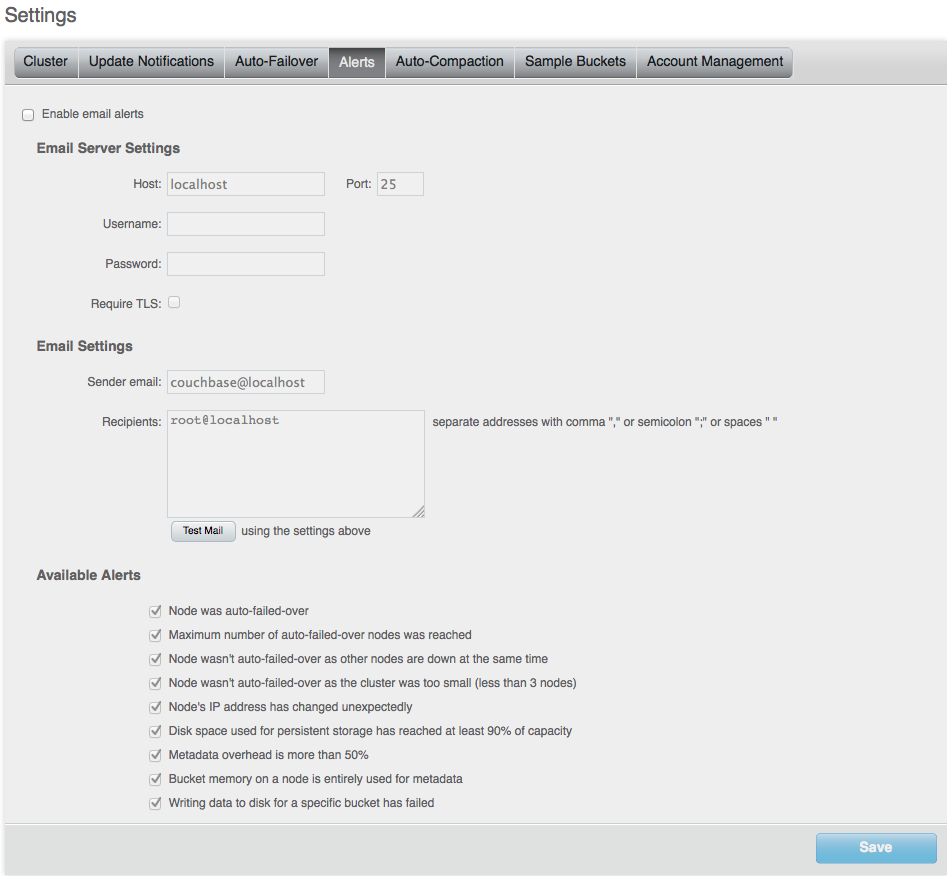
For more information on Auto-Failover, see Using Automatic Failover.
Enabling auto-compaction
The Auto-Compaction tab configures the default auto-compaction settings for
all the databases. These can be overridden using per-bucket settings available
within Creating and Editing Data
Buckets. For
information about changing these settings with the REST API, see the
REST API, Setting Auto-Compaction.
You can provide a purge interval to remove the key and metadata for items that have been deleted or are expired. This is known as ‘tombstone purging’. For background information, see Introduction, Tombstone Purging.
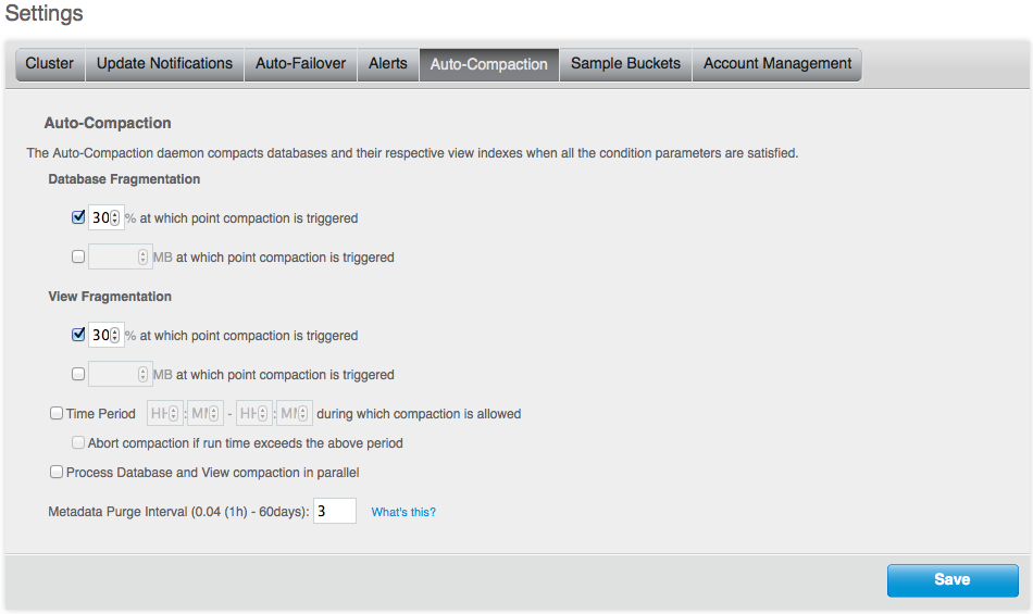
The settings tab sets the following default parameters:
-
Database FragmentationIf checked, you must specify either the percentage of fragmentation at which database compaction will be triggered, or the database size at which compaction will be triggered. You can also configure both trigger parameters.
-
View FragmentationIf checked, you must specify either the percentage of fragmentation at which database compaction will be triggered, or the view size at which compaction will be triggered. You can also configure both trigger parameters.
-
Time PeriodIf checked, you must specify the start hour and minute, and end hour and minute of the time period when compaction is allowed to occur.
-
Abort if run time exceeds the above periodIf checked, if database compaction is running when the configured time period ends, the compaction process will be terminated.
-
Process Database and View compaction in parallelIf enabled, database and view compaction will be executed simultaneously, implying a heavier processing and disk I/O load during the compaction process.
-
Metadata Purge IntervalDefaults to three days. Tombstones are records of expired or deleted items and they include the key and metadata. Tombstones are used in Couchbase Server to provide eventual consistency of data between clusters.
The auto-compaction process waits this number of days before it permanently deletes tombstones for expired or deleted items.
If you set this value too low, you may see more inconsistent results in views queries such as deleted items in a result set. You may also see inconsistent items in clusters with XDCR set up between the clusters. If you set this value too high, it will delay the server from reclaiming disk space.
You can also change this setting with the REST API, see the REST API, Setting Auto-Compaction.
For more information on compaction, see Database and View Compaction. For information on how auto-compaction operates, see Auto-Compaction Configuration.
Installing sample buckets
The Sample Buckets tab enables you to install the sample bucket data if the
data has not already been loaded in the system. For more information on the
sample data available, see Couchbase Sample Buckets.
If the sample bucket data was not loaded during setup, select the sample buckets that you want to load using the checkboxes, and click Create.
If the sample bucket data has already been loaded, it will be listed under the
Installed Samples section of the page.
Account management settings
Account management settings allows you to set up and modify the read-only user’s user name and password. This user has read-only access and cannot make any changes to the system. The user can only view existing servers, buckets, views and monitor stats.
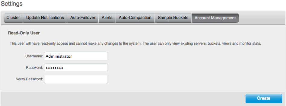
Updating notifications
During installation you can select to enable the Update Notification function. Update notifications allow a client accessing the Couchbase Web Console to determine whether a newer version of Couchbase Server is available for download.
If you select the Update Notifications option, the Web Console will
communicate with Couchbase servers to confirm the version number of your
Couchbase installation. During this process, the client submits the following
information to the Couchbase server:
The current version of your Couchbase Server installation. When a new version of Couchbase Server becomes available, you will be provided with notification of the new version and information on where you can download the new version.
Basic information about the size and configuration of your Couchbase cluster. This information will be used to help us prioritize our development efforts.
You can enable/disable software update notifications
Note
The process occurs within the browser accessing the web console, not within the server itself, and no further configuration or internet access is required on the server to enable this functionality. Provided that the client accessing the Couchbase server console has internet access, the information can be communicated to the Couchbase servers.
The update notification processes the information anonymously, and the data cannot be tracked. The information is only used to provide you with updated notification and to provide information that will help us improve the future development process for Couchbase Server and related products.
If the browser or computer that you are using to connect to your Couchbase Server web console does not have Internet access, the update notification system will not work.
Notifications
If an update notification is available, the counter within the button display within the Couchbase Console will be displayed with the number of available updates.
Viewing Available Updates
To view the available updates, click on the Settings link. This displays your
current version and update availability. From here you can be taken to the
download location to obtain the updated release package.
Warnings and alerts
A new alerting systems has been built into the Couchbase Web Console. This is sued to highlight specific issues and problems that you should be aware of and may need to check to ensure the health of your Couchbase cluster.
Alerts are provided as a popup within the web console. A sample of the IP address popup is shown below:
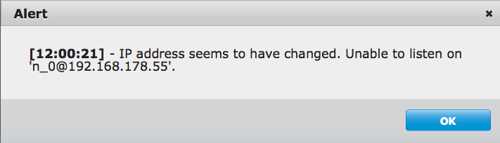
The following errors and alerts are supported:
-
IP Address Changes
If the IP address of a Couchbase Server in your cluster changes, you will be warned that the address is no longer available. You should check the IP address on the server, and update your clients or server configuration.
-
OOM (Hard)
Indicates if the bucket memory on a node is entirely used for metadata.
-
Commit Failure
Indicates that writing data to disk for a specific bucket has failed.
-
Metadata Overhead
Indicates that a bucket is now using more than 50% of the allocated RAM for storing metadata and keys, reducing the amount of RAM available for data values.
-
Disk Usage
Indicates that the available disk space used for persistent storage has reached at least 90% of capacity.
Admin tasks
For general running and configuration, Couchbase Server is self-managing. The management infrastructure and components of the Couchbase Server system are able to adapt to the different events within the cluster. There are only a few different configuration variables. The majority of these configuration variables do not need to be modified or altered in most installations.
However, there are a number of different tasks that are performed over the lifetime of the cluster environment including:
- Expand your cluster when you need to expand the RAM or disk I/O capabilities.
- Failover and altering the size of your cluster as your application demands change.
- Monitoring and reacting to the various statistics reported by the server to ensure that your cluster is operating at the highest performance level.
- Backing up the cluster.
Increasing or reducing your cluster size
When your cluster requires additional RAM, disk I/O or network capacity, you will need to expand the size of your cluster. If the increased load is only a temporary event, then you may later want to reduce the size of your cluster.
You can add or remove multiple nodes from your cluster at the same time. Once
the new node arrangement has been configured, the process redistributing the
data and bringing the nodes into the cluster is called rebalancing. The
rebalancing process moves the data around the cluster to match the new
structure, and can be performed live while the cluster is still servicing
application data requests.
More information on increasing and reducing your cluster size and performing a rebalance operation is available in Rebalancing.
Warming up a server There may be cases where you want to explicitly shutdown a server and then restart it. Typically the server had been running for a while and has data stored on disk when you restart it. In this case, the server needs to undergo a warmup process before it can again serve data requests. To manage the warmup process for Couchbase Server instances, see Handling Server Warmup.
Handling a failover situation
A failover situation occurs when one of the nodes within your cluster fails, usually due to a significant hardware or network problem. Couchbase Server is designed to cope with this situation through the use of replicas which provide copies of the data around the cluster which can be activated when a node fails.
Couchbase Server provides two mechanisms for handling failover. Automated Failover allows the cluster to operate autonomously and react to failovers without human intervention. Monitored failover enables you to perform a controlled failure by manually failing over a node. There are additional considerations for each failover type, and you should read the notes to ensure that you know the best solution for your specific situation.
For more information, see Failing Over Nodes.
Managing database and view fragmentation
The database and view index files created by Couchbase Server can become fragmented. This can cause performance problems, as well as increasing the space used on disk by the files, compared to the size of the information they hold. Compaction reduces this fragmentation to reclaim the disk space.
Information on how to enable and configure auto-compaction is available in Database and View Compaction.
Backing up and restoring your cluster data
Couchbase Server automatically distributes your data across the nodes within the cluster, and supports replicas of that data. It is good practice, however, to have a backup of your bucket data in the event of a more significant failure.
More information on the available backup and restore methods are available in Backup and Restore.
Read-Only users
As of Couchbase Server 2.2+ you can create one non-administrative user who has read-only access in the Web Console and the REST API. A read-only user cannot create buckets, edit buckets, add nodes to clusters, change XDCR settings, create views or see any stored data. Any REST API calls which require an administrator will fail and return an error for this user. In the Web Console a read-only user will be able to view:
- Cluster Overview.
- Design documents and view definitions but cannot query views.
- Bucket summaries including Cache Size and Storage Size, but cannot view documents.
- List of XDCR replications and remote clusters.
- Logged events under the Log tab, but the user cannot Generate Diagnostic Report.
- Settings for a cluster.
The read-only user will not be able to set up a Couchbase SDK to connect to the server. All SDKs require that a client connect with bucket-level credentials. For more information about Couchbase SDKs, see Couchbase, All Client Libraries.
To create a read-only user:
- In Couchbase Web Console, click Settings. A panel appears with several different sub-tabs.
-
Click Account Management. A panel appears where you can add a read-only user:
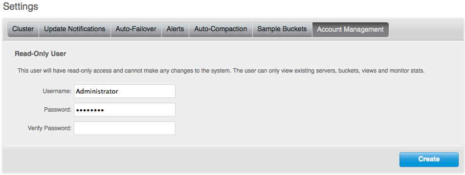
Enter a Username, Password and verify the password.
- Click Create. The panel refreshes and has options for resetting the read-only user password or deleting the user:
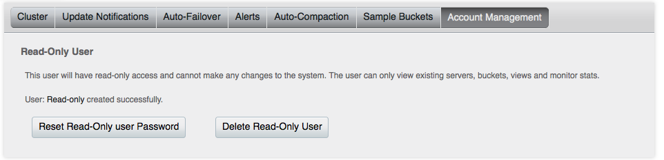
This read-only user can now log into Couchbase Web Console in read-only mode or perform REST API GET requests that do not require administrative credentials. If a read-only user performs a REST POST or DELETE request that changes cluster, bucket, XDCR, or node settings, the server will send an HTTP 401 error:
HTTP/1.1 401 Unauthorized
WWW-Authenticate: Basic realm="Couchbase Server Admin / REST"
....
For more information about Web Console or REST API, see Using the Web Console or the REST API. You can also create a read-only user with the REST API, see Creating Read-Only Users.
Using multi-readers and writers
Multiple readers and writers are supported to persist data onto disk. For earlier versions of Couchbase Server, each bucket instance had only single disk reader and writer workers. By default this is set to three total workers per data bucket, with two reader workers and one writer worker for the bucket. This feature can help you increase your disk I/O throughput. If your disk utilization is below the optimal level, you can increase the setting to improve disk utilization. If your disk utilization is near the maximum and you see heavy I/O contention, you can decrease this setting. By default we allocate three total readers and writers.
How you change this setting depends on the hardware in your Couchbase cluster:
If you deploy your cluster on the minimum hardware requirement which is dual-core CPUs running on 2GHz and 4GB of physical RAM, you should stay with the default setting of three.
If you deploy your servers on recommended hardware requirements or above you can increase this setting to eight. The recommended hardware requirements are quad-core processes on 64-bit CPU and 3GHz, 16GB RAM physical storage. We also recommend solid state drives.
If you have a hardware configuration which conforms to pre-2.1 hardware requirements, you should change this setting to the minimum, which is two (2) workers per data bucket.
For more information about system requirements for Couchbase Server, see Resource Requirements.
Changing the Number of Readers and Writers
You should configure this setting in Couchbase Web Console when you initially create a data bucket. For general information on creating buckets, see Creating a New Bucket.
-
Under Data Buckets, click Create New Data Bucket.
A Configure Bucket panel appears where you can provide settings for the new bucket.
-
Select a number of reader/writers under Disk Read-Write Concurrency.
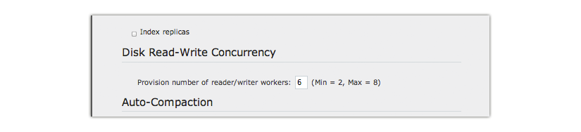
Provide other bucket-level settings of your choice.
-
Click Create.
The new bucket will appear under the Data Buckets tabs in Web Console with a yellow indicator to show the bucket is in warmup phase:
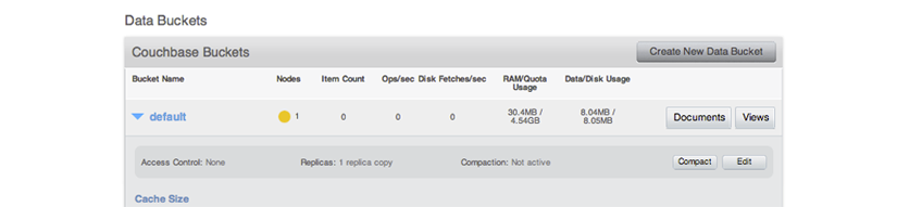
After the bucket completes warmup, it will appear with a green indicator next to it:

This default bucket is now ready to receive and serve requests. If you create a named bucket, you will see a similar status indicator next to your named bucket.
Viewing Status of Multi- Readers and Writers
After you change this setting you can view the status of this setting with
cbstats :
/opt/couchbase/bin/cbstats hostname:11210 -b bucket_name raw workload
ep_workload:num_readers: 3
ep_workload:num_shards: 3
ep_workload:num_writers: 2
ep_workload:policy: Optimized for read data access
This indicates we have three reader threads and two writer threads on
bucket_name in the cluster at hostname:11210. The vBucket map for the data
bucket is grouped into multiple shards, where one read worker will access one of
the shards. In this example we have one reader for each of the three shards.
This report also tell us we are optimized for read data access because we have
more reader threads than writer threads for the bucket. You can also view the
number of threads if you view the data bucket properties via a REST call:
curl -u Admin:password http://localhost:8091/pools/default/buckets/bucket_name
This provides information about the named bucket as a JSON response, including the total number of threads:
{"name":"bucket_name","bucketType":"couchbase"
....
"replicaNumber":1,
"threadsNumber":5,
....
}
To view the changed behavior, go to the Data Buckets tab and select your named
bucket. Under the summary section, you can view the disk write queue for
change in drain rate. Under the Disk Queues section, you see a change in the
active and replica drain rate fields after you change this setting. For more
information about bucket information in Web Console, see Individual Bucket
Monitoring.
Changing Readers and Writers for Existing Buckets
You can change this setting after you create a data bucket in Web Console or REST API. If you do so, the bucket will be re-started and will go through server warmup before it becomes available. For more information about warmup, see Handling Server Warmup.
To change this setting in Web Console:
-
Click the Data Buckets tab.
A table with all data buckets in your cluster appears.
-
Click the drop-down next to your data bucket.
General information about the bucket appears as well as controls for the bucket.
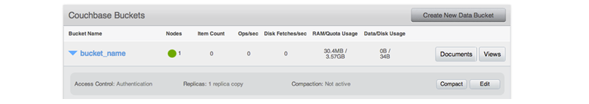
-
Click Edit.
A Configure Bucket panel appears where you can edit the current settings for the bucket. The Disk Read-Write section is where you will change this setting.
Enter a number of readers and writers.
-
Click Save.
A warning appears indicating that this change will recreate the data bucket.

-
Click Continue
The Data Buckets tab appears and you see the named bucket with a yellow indicator. This tells you the bucket is recreated and is warming up. The indicator turns green when the bucket has completed warmup. At this point it is ready to receive and serve requests.
To change this setting via REST, we provide the threadsNumber parameter with a
value from two to eight. The following is an example REST call:
curl -X POST -u Admin:password http://10.3.3.72:8091/pools/default/buckets/bucket_name -d \
ramQuotaMB=4000 -d threadsNumber=3 -v
For details about changing bucket properties via REST, including limitations and behavior, see Creating and Editing Data Buckets.
You see the following request via HTTP:
About to connect() to 10.3.3.72 port 8091 (#0)
Trying 10.3.3.72... connected
Connected to 10.3.3.72 (10.3.3.72) port 8091 (#0)
Server auth using Basic with user 'Administrator'
POST /pools/default/buckets/bucket_name HTTP/1.1
....
Upon success you will see this response:
HTTP/1.1 200 OK
....
If you provide an invalid number of threads, you will a response similar to the following:
HTTP/1.1 400 Bad Request
....
{"errors":{"threadsNumber":"The number of threads can't be greater than 8"},"
If you upgrade a Couchbase cluster, a new node can use this setting without bucket restart and warmup. In this case you set up a new 2.1 or higher node, add that node to the cluster, and on that new node edit the existing bucket setting for readers and writers. After you rebalance the cluster, this new node will perform reads and writes with multiple readers and writers and the data bucket will not restart or go through warmup. All existing pre-2.1 nodes will remain with a single readers and writers for the data bucket. As you continue the upgrade and add additional 2.1 or higher nodes to the cluster, these new nodes will automatically pick up the setting and use multiple readers and writers for the bucket. For general information about Couchbase cluster upgrade, see Upgrading to Couchbase Server.
Handling server warmup
Couchbase Server provides improved performance for server warmup ; this is the process a restarted server must undergo before it can serve data. During this process the server loads items persisted on disk into RAM. One approach to load data is to do sequential loading of items from disk into RAM; however it is not necessarily an effective process because the server does not take into account whether the items are frequently used. In Couchbase Server, additional optimizations is provided during the warmup process to make data more rapidly available, and to prioritize frequently-used items in an access log. The server pre-fetches a list of most-frequently accessed keys and fetches these documents before it fetches any other items from disk.
The server also runs a configurable scanner process which will determine which keys are most frequently-used. You can use Couchbase Server command-line tools to change the initial time and the interval for the process. You may want to do this for instance, if you have a peak time for your application when you want the keys used during this time to be quickly available after server restart. For more information, see Changing access log settings.
The server can also switch into a ready mode before it has actually retrieved all documents for keys into RAM, and therefore can begin serving data before it has loaded all stored items. This is also a setting you can configure so that server warmup is faster.
The following describes the initial warmup phases for the Couchbase Server. In these first phase, the server begins fetch all keys and metadata from disk. Then the server gets access log information it needs to retrieve the most-used keys:
Initialize. At this phase, the server does not have any data that it can serve yet. The server starts populating a list of all vBuckets stored on disk by loading the recorded, initial state of each vBucket.
Key Dump. In this next phase, the server begins pre-fetching all keys and metadata from disk based on items in the vBucket list.
Check Access Logs. The server then reads a single cached access log which indicates which keys are frequently accessed. The server generates and maintains this log on a periodic basis and it can be configured. If this log exists, the server will first load items based on this log before it loads other items from disk.
Once Couchbase Server has information about keys and has read in any access log information, it is ready to load documents:
Loading based on Access Logs Couchbase Server loads documents into memory based on the frequently-used items identified in the access log.
Loading Data. If the access log is empty or is disabled, the server will sequentially load documents for each key based on the vBucket list.
Couchbase Server is able to serve information from RAM when one of the following conditions is met during warmup:
The server has finished loading documents for all keys listed in the access log, or
The server has finished loading documents for every key stored on disk for all vBuckets, or
The percentage of documents loaded into memory is greater than, or equal to, the setting for
ep_warmup_min_items_threshold, orIf total % of RAM filled by documents is greater than, or equal to, the setting for
ep_warmup_min_memory_threshold, orIf total RAM usage by a node is greater than or equal to the setting for
mem_low_wat.
When the server reaches one of these states, this is known as the run level ; when Couchbase Server reaches this point, it immediately stops loading documents for the remaining keys. After this point, Couchbase Server will load this remaining documents from disk into RAM as a background data fetch.
In order to adjust warmup behavior, it is also important for you to understand the access log and scanning process in Couchbase Server. The server uses the access log to determine which documents are most frequently used, and therefore which documents should be loaded first.
The server has a process that will periodically scan every key in RAM and
compile them into a log, named access.log as well as maintain a backup of this
access log, named access.old. The server can use this backup file during
warmup if the most recent access log has been corrupted during warmup or node
failure. By default this process runs initially at 2:00 GMT and will run again
in 24- hour time periods after that point. You can configure this process to run
at a different initial time and at a different fixed interval.
If a client tries to contact Couchbase Server during warmup, the server will
produce a ENGINE_TMPFAIL (0x0d) error code. This error indicates that data
access is still not available because warmup has not yet finished. For those of
you who are creating your own Couchbase SDK, you will need to handle this error
in your library. This may mean that the client waits and retries, or the client
performs a backoff of requests, or it produces an error and does not retry the
request. For those of you who are building an application with a Couchbase SDK,
be aware that how this error is delivered and handled is dependent upon the
individual SDKs. For more information, refer to the Language Reference for your
chosen Couchbase SDK.
Getting warmup information
You can use cbstats to get information about server warmup, including the
status of warmup and whether warmup is enabled. The following are two alternates
to filter for the information:
> cbstats localhost:11210 -b beer-sample -p bucket_password all | grep 'warmup'
> cbstats hostname:11210 -b my_bucket -p bucket_password raw warmup
Here the localhost:11210 is the host name and default memcached port for a
given node and beer-sample is a named bucket for the node. If you do not
specify a bucket name, the command will apply to any existing default bucket for the node.
- ep_warmup_thread - Indicates whether the warmup completed or is still running. Returns “running” or “complete”.
-
ep_warmup_state - Indicates the current progress of the warmup:
- Initial - Start warmup processes.
- EstimateDatabaseItemCount - Estimate database item count.
- KeyDump - Begin loading keys and metadata based, but not documents, into RAM.
- CheckForAccessLog - Determine if an access log is available. This log indicates which keys have been frequently read or written.
- LoadingAccessLog - Load information from access log.
- LoadingData* - The server is loading data first for keys listed in the access log, or if no log available, based on keys found during the ‘Key Dump’ phase.
- Done - The server is ready to handle read and write requests.
Be aware that this tool is a per-node, per-bucket operation. That means that if you want to perform this operation, you must specify the IP address of a node in the cluster and a named bucket. If you do not provided a named bucket, the server will apply the setting to any default bucket that exists at the specified node. If you want to perform this operation for an entire cluster, you will need to perform the command for every node/bucket combination that exists for that cluster.
There are more detailed statistics available on the warmup process. For more information, see Getting warmup information.
Changing the warmup threshold
To modify warmup behavior by changing the setting for
ep_warmup_min_items_threshold use the command-line tool provided with your
Couchbase Server installation, cbepctl. This indicates the percentage of items
loaded in RAM that must be reached for Couchbase Server to begin serving data.
The lower this number, the sooner your server can begin serving data. Be aware,
however that if you set this value to be too low, once requests come in for
items, the item may not be in memory and Couchbase Server will experience
cache-miss errors.
Changing access scanner settings
The server runs a periodic scanner process which will determine which keys are
most frequently-used, and therefore, which documents should be loaded first
during server warmup. You can use cbepctl flush_param to change the initial
time and the interval for the process. You may want to do this, for instance, if
you have a peak time for your application when you want the keys used during
this time to be quickly available after server restart.
Note
If you want to change this setting for an entire Couchbase cluster, you
will need to perform this command on per-node and per-bucket in the cluster. By
default, any setting you change with cbepctl will only be for the named bucket
at the specific node you provide in the command.
This means that if you have a data bucket that is shared by two nodes, you will nonetheless need to issue this command twice and provide the different host names and ports for each node and the bucket name. Similarly, if you have two data buckets for one node, you need to issue the command twice and provide the two data bucket names. If you do not specify a named bucket, it will apply to the default bucket or return an error if a default bucket does not exist.
By default the scanner process runs once every 24 hours with a default initial start time of 2:00 AM UTC. This means after you install a new Couchbase Server instance or restart the server, by default the scanner will run every 24- hour time period at 2:00 AM UTC by default. To change the time interval when the access scanner process runs to every 20 minutes:
> ./cbepctl localhost:11210 -b beer-sample set flush_param alog_sleep_time 20
This updates the parameter for the named bucket, beer-sample on the given node
on localhost. To change the initial time that the access scanner process runs
from the default of 2:00 AM UTC:
> ./cbepctl hostname:11210 -b beer-sample -p beer_password set flush_param alog_task_time 13
In this example we set the initial time to 1:00 PM UTC.
Be aware that this tool is a per-node, per-bucket operation. That means that if you want to perform this operation, you must specify the IP address of a node in the cluster and a named bucket. If you do not provided a named bucket, the server will apply the setting to any default bucket that exists at the specified node. If you want to perform this operation for an entire cluster, you will need to perform the command for every node/bucket combination that exists for that cluster. For more information, see cbepctl tool.
Handling replication within a cluster
Within a Couchbase cluster, you have replica data which is a copy of an item at another node. After you write an item to Couchbase Server, it makes a copy of this data from the RAM of one node to another node. Distribution of replica data is handled in the same way as active data; portions of replica data will be distributed around the Couchbase cluster onto different nodes to prevent a single point of failure. Each node in a cluster will have replica data and active data ; replica data is the copy of data from another node while active data is data that had been written by a client on that node.
Replication of data between nodes is entirely peer-to-peer based; information will be replicated directly between nodes in the cluster. There is no topology, hierarchy or master-slave relationship between nodes in a cluster. When a client writes to a node in the cluster, Couchbase Server stores the data on that node and then distributes the data to one or more nodes within a cluster. The following shows two different nodes in a Couchbase cluster, and illustrates how two nodes can store replica data for one another:
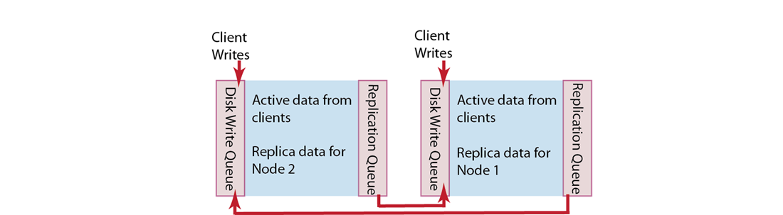
When a client application writes data to a node, that data will be placed in a replication queue and then a copy will be sent to another node. The replicated data will be available in RAM on the second node and will be placed in a disk write queue to be stored on disk at the second node.
Notice that a second node will also simultaneously handle both replica data and incoming writes from a client. The second node will put both replica data and incoming writes into a disk write queue. If there are too many items in the disk write queue, this second node can send a backoff message to the first node. The first node will then reduce the rate at which it sends items to the second node for replication. This can sometimes be necessary if the second node is already handling a large volume of writes from a client application. For information about changing this setting, see Changing Disk Write Queue Quotas.
If multiple changes occur to the same document waiting to be replicated, Couchbase Server is able to de-duplicate, or ‘de-dup’ the item; this means for the sake of efficiency, it will only send the latest version of a document to the second node.
If the first node fails in the system the replicated data is still available at the second node. Couchbase can serve replica data from the second node nearly instantaneously because the second node already has a copy of the data in RAM; there is no need for the data to be copied over from the failed node or to be fetched from disk. Once replica data is enabled at the second node, Couchbase Server updates a map indicating where the data should be retrieved, and the server shares this information with client applications. Client applications can then get the replica data from the functioning node. For more information about node failure and failover, see Failover Nodes.
Providing data replication
You can configure data replication for each bucket in cluster. You can also configure different buckets to have different levels of data replication, depending how many copies of your data you need. For the highest level of data redundancy and availability, you can specify that a data bucket will be replicated three times within the cluster.
Replication is enabled once the number of nodes in your cluster meets the number of replicas you specify. For example, if you configure three replicas for a data bucket, replication will only be enabled once you have four nodes in the cluster.
Note
After you specify the number of replicas you want for a bucket and then create the bucket, you cannot change this value. Therefore be certain you specify the number of replicas you truly want.
For more information about creating and editing buckets, or specifying replicas for buckets, see Creating and Editing Data Buckets.
Specifying backoff for replication
Your cluster is set up to perform some level of data replication between nodes within the cluster for any given node. Every node will have both active data and replica data. Active data is all the data that had been written to the node from a client, while replica data is a copy of data from another node in the cluster. Data replication enables high availability of data in a cluster. Should any node in cluster fail, the data will still be available at a replica.
On any give node, both active and replica data must wait in a disk write queue before being written to disk. If your node experiences a heavy load of writes, the replication queue can become overloaded with replica and active data waiting to be persisted.
By default a node will send backoff messages when the disk write queue on the
node contains one million items or 10%. When other nodes receive this message,
they will reduce the rate at which they send replica data. You can configure
this default to be a given number so long as this value is less than 10% of the
total items currently in a replica partition. For instance if a node contains 20
million items, when the disk write queue reaches 2 million items a backoff
message will be sent to nodes sending replica data. You use the Couchbase
command-line tool, cbepctl to change this configuration:
> ./cbepctl 10.5.2.31:11210 -b bucket_name -p bucket_password set tap_param tap_throttle_queue_cap 2000000
In this example we specify that a node sends replication backoff requests when it has two million items or 10% of all items, whichever is greater. You will see a response similar to the following:
setting param: tap_throttle_queue_cap 2000000
In this next example, we change the default percentage used to manage the replication stream. If the items in a disk write queue reach the greater of this percentage or a specified number of items, replication requests will slow down:
> ./cbepctl 10.5.2.31:11210 set -b bucket_name tap_param tap_throttle_cap_pcnt 15
In this example, we set the threshold to 15% of all items at a replica node. When a disk write queue on a node reaches this point, it will send replication backoff requests to other nodes.
Be aware that this tool is a per-node, per-bucket operation. That means that if you want to perform this operation, you must specify the IP address of a node in the cluster and a named bucket. If you do not provided a named bucket, the server will apply the setting to any default bucket that exists at the specified node. If you want to perform this operation for an entire cluster, you will need to perform the command for every node/bucket combination that exists for that cluster.
For more information about changing this setting, see cbepctl Tool. You can also monitor the progress of this backoff operation in Couchbase Web Console under Tap Queue Statistics | back-off rate. For more information, see Monitoring TAP Queues.
Ejection and working set management
Couchbase Server actively manages the data stored in a caching layer; this includes the information which is frequently accessed by clients and which needs to be available for rapid reads and writes. When there are too many items in RAM, Couchbase Server removes certain data to create free space and to maintain system performance. This process is called “working set management” and the set of data in RAM is referred to as the “working set”.
In general the working set consists of all the keys, metadata, and associated documents which are frequently used require fast access. The process the server performs to remove data from RAM is known as ejection. When the server performs this process, it removes the document, but not the keys or metadata for the item. Keeping keys and metadata in RAM serves three important purposes in a system:
Couchbase Server uses the remaining key and metadata in RAM if a request for that key comes from a client. If a request occurs, the server then tries to fetch the item from disk and return it into RAM.
The server can also use the keys and metadata in RAM for “miss access”. This means that it is quickly determine whether an item is missing and if so, perform some action, such as add it.
Finally, the expiration process in Couchbase Server uses the metadata in RAM to quickly scan for items that are expired and later remove them from disk. This process is known as the “expiry pager” and runs every 60 minutes by default. For more information about the pager, and changing the setting for it, see Changing the Disk Cleanup Interval.
Not-Frequently-Used Items
All items in the server contain metadata indicating whether the item has been recently accessed or not. This metadata is known as not-recently-used (NRU). If an item has not been recently used, then the item is a candidate for ejection if the high water mark has been exceeded. When the high water mark has been exceeded, the server evicts items from RAM.
Couchbase Server provides two NRU bits per item and also provides a replication protocol that can propagate items that are frequently read, but not mutated often.
For earlier versions, Couchbase Server provided only a single bit for NRU and a different replication protocol which resulted in two issues: metadata could not reflect how frequently or recently an item had been changed, and the replication protocol only propagated NRUs for mutation items from an active vBucket to a replica vBucket. This second behavior meant that the working set on an active vBucket could be quite different than the set on a replica vBucket. By changing the replication protocol, the working set in replica vBuckets will be closer to the working set in the active vBucket.
NRUs are decremented or incremented by server processes to indicate an item is more frequently used, or less frequently used. Items with lower bit values have lower scores and are considered more frequently used. The bit values, corresponding scores and status are as follows:
| Binary NRU | Score | Working Set Replication Status (WSR) | Access Pattern | Description |
|---|---|---|---|---|
| 00 | 0 | TRUE | Set by write access to 00. Decremented by read access or no access. | Most heavily used item. |
| 01 | 1 | Set to TRUE | Decremented by read access. | Frequently access item. |
| 10 | 2 | Set to FALSE | Initial value or decremented by read access. | Default for new items. |
| 11 | 3 | Set to FALSE | Incremented by item pager for eviction. | Less frequently used item. |
When WSR is set to TRUE it means that an item should be replicated to a replica vBucket. There are two processes which change the NRU for an item:
- A client reads or writes an item, the server decrements NRU and lowers the item’s score
- A daily process which creates a list of frequently-used items in RAM. After this process runs, the server increments one of the NRU bits.
Because the two processes changes NRUs, they also affect which items are candidates for ejection. For more information about the access scanner, see Handling Server Warmup.
Couchbase Server settings can be adjusted to change behavior during ejection. For example, specify the percentage of RAM to be consume before items are ejected or specify whether ejection should occur more frequently on replicated data than on original data. Couchbase recommends that the default settings be used.
Understanding the Item Pager
The item pager process, which runs periodically, removes documents from RAM and retains the item’s key and metadata. If the amount of RAM used by items reaches the high water mark (upper threshold), both active and replica data are ejected until the memory usage (amount of RAM consumed) reaches the low water mark (lower threshold). Evictions of active and replica data occur with the ratio probability of 40% (active data) to 60% (replica data) until the memory usage reaches the low watermark. Both the high water mark and low water mark are expressed as a percentage amount of RAM, such as 80%.
Both the high water mark and low water mark can be changed by providing a percentage amount of RAM for a node, for example, 80%. Couchbase recommends that the following default settings be used:
| Version | High Water Mark | Low Water Mark |
|---|---|---|
| 2.0 | 75% | 60% |
| 2.0.1 and higher | 85% | 75% |
The item pager ejects items from RAM in two phases:
Phase 1: Eject based on NRU. Scan NRU for items and create list of all items with score of 3. Eject all items with a NRU score of 3. Check RAM usage and repeat this process if usage is still above the low water mark.
Phase 2: Eject based on Algorithm. Increment all item NRUs by 1. If an NRU is equal to 3, generate a random number and eject that item if the random number is greater than a specified probability. The probability is based on current memory usage, low water mark, and whether a vBucket is in an active or replica state. If a vBucket is in active state the probability of ejection is lower than if the vBucket is in a replica state. The default probabilities for ejection from active of replica vBuckets is as follows:
The following is the probability of ejection based on active vs. replica vBuckets:
| Active vBucket | Replica vBucket |
|---|---|
| 60% | 40% |
For instructions to change this setting, see Changing thresholds for ejection.
Database and view compaction
The data files in which information is stored in a persistent state for a Couchbase Bucket are written to and updated as information is appended, updated and deleted. This process can eventually lead to gaps within the data file (particularly when data is deleted) which can be reclaimed using a process called compaction.
The index files that are created each time a view is built are also written in a sequential format. Updated index information is appended to the file as updates to the stored information is indexed.
In both these cases, frequent compaction of the files on disk can help to reclaim disk space and reduce fragmentation.
Compaction process
How it works
Couchbase compacts views and data files. For database compaction, a new file is created into which the active (non-stale) information is written. Meanwhile, the existing database files stay in place and continue to be used for storing information and updating the index data. This process ensures that the database continues to be available while compaction takes place. Once compaction is completed, the old database is disabled and saved. Then any incoming updates continue in the newly created database files. The old database is then deleted from the system.
View compaction occurs in the same way. Couchbase creates a new index file for each active design document. Then Couchbase takes this new index file and writes active index information into it. Old index files are handled in the same way old data files are handled during compaction. Once compaction is complete, the old index files are deleted from the system.
How to use it
Compaction takes place as a background process while Couchbase Server is running. You do not need to shutdown or pause your database operation, and clients can continue to access and submit requests while the database is running. While compaction takes place in the background, you need to pay attention to certain factors.
Make sure you perform compaction…
… on every server: Compaction operates on only a single server within your Couchbase Server cluster. You will need to perform compaction on each node in your cluster, on each database in your cluster.
-
… during off-peak hours: The compaction process is both disk and CPU intensive. In heavy-write based databases where compaction is required, the compaction should be scheduled during off-peak hours (use auto-compact to schedule specific times).
If compaction isn’t scheduled during off-peak hours, it can cause problems. Because the compaction process can take a long to complete on large and busy databases, it is possible for the compaction process to fail to complete properly while the database is still active. In extreme cases, this can lead to the compaction process never catching up with the database modifications, and eventually using up all the disk space. Schedule compaction during off-peak hours to prevent this!
-
… with adequate disk space: Because compaction occurs by creating new files and updating the information, you may need as much as twice the disk space of your current database and index files for compaction to take place.
However, it is important to keep in mind that the exact amount of the disk space required depends on the level of fragmentation, the amount of dead data and the activity of the database, as changes during compaction will also need to be written to the updated data files.
Before compaction takes place, the disk space is checked. If the amount of available disk space is less than twice the current database size, the compaction process does not take place and a warning is issued in the log. See Log.
Compaction Behavior
Stop/Restart: The compaction process can be stopped and restarted. However, you should be aware that the if the compaction process is stopped, further updates to database are completed, and then the compaction process is restarted, the updated database may not be a clean compacted version. This is because any changes to the portion of the database file that were processed before the compaction was canceled and restarted have already been processed.
Auto-compaction: Auto-compaction automatically triggers the compaction process on your database. You can schedule specific hours when compaction can take place.
-
Compaction activity log: Compaction activity is reported in the Couchbase Server log. You will see entries similar to following showing the compaction operation and duration:
-
Compaction activity log: Compaction activity is reported in the Couchbase Server log. You can see the following items for compaction:
Autocompaction Indicates compaction cannot be performed because of inadequate disk space
-
Manually triggered compaction
- Compaction completed successfully
- Compaction failed
-
Purge deletes compaction
- Compaction started/completed
- Compaction failed
For information on accessing the log, see Log.
-
Auto-compaction configuration
Couchbase Server incorporates an automated compaction mechanism that can compact both data files and the view index files, based on triggers that measure the current fragmentation level within the database and view index data files.
Note
Spatial indexes are not automatically compacted. Spatial indexes must be compacted manually.
Auto-compaction can be configured in two ways:
Default Auto-Compaction affects all the Couchbase Buckets within your Couchbase Server. If you set the default Auto-Compaction settings for your Couchbase server then auto-compaction is enabled for all Couchbase Buckets automatically. For more information, see Settings.
Bucket Auto-Compaction can be set on individual Couchbase Buckets. The bucket-level compaction always overrides any default auto-compaction settings, including if you have not configured any default auto-compaction settings. You can choose to explicitly override the Couchbase Bucket specific settings when editing or creating a new Couchbase Bucket. See Creating and Editing Data Buckets.
The available settings for both default Auto-Compaction and Couchbase Bucket specific settings are identical:
-
Database Fragmentation
The primary setting is the percentage level within the database at which compaction occurs. The figure is expressed as a percentage of fragmentation for each item, and you can set the fragmentation level at which the compaction process will be triggered.
For example, if you set the fragmentation percentage at 10%, the moment the fragmentation level has been identified, the compaction process will be started, unless you have time limited auto-compaction. SeeTime Period.
-
View Fragmentation
The View Fragmentation specifies the percentage of fragmentation within all the view index files at which compaction will be triggered, expressed as a percentage.
-
Time Period
To prevent auto compaction taking place when your database is in heavy use, you can configure a time during which compaction is allowed. This is expressed as the hour and minute combination between which compaction occurs. For example, you could configure compaction to take place between 01:00 and 06:00.
If compaction is identified as required outside of these hours, compaction will be delayed until the specified time period is reached.
Note
The time period is applied every day while the Couchbase Server is active. The time period cannot be configured on a day-by-day basis.
-
Compaction abortion
The compaction process can be configured so that if the time period during which compaction is allowed ends while the compaction process is still completing, the entire compaction process will be terminated. This option affects the compaction process:
-
Enabled
If this option is enabled, and compaction is running, the process will be stopped. The files generated during the compaction process will be kept, and compaction will be restarted when the next time period is reached.
This can be a useful setting if want to ensure the performance of your Couchbase Server during a specified time period, as this will ensure that compaction is never running outside of the specified time period.
-
Disabled
If compaction is running when the time period ends, compaction will continue until the process has been completed.
Using this option can be useful if you want to ensure that the compaction process completes.
-
-
Parallel Compaction
By default, compaction operates sequentially, executing first on the database and then the Views if both are configured for auto-compaction. If you enable parallel compaction, both the databases and the views can be compacted at the same time. This requires more CPU and database activity for both to be processed simultaneously, but if you have CPU cores and disk I/O (for example, if the database and view index information is stored on different physical disk devices), the two can complete in a shorter time.
-
Metadata Purge Interval
You can remove tombstones for expired and deleted items as part of the auto-compaction process. Tombstones are records containing the key and metadata for deleted and expired items and are used for eventually consistency between clusters and for views.
Configuration of auto-compaction is through Couchbase Web Console. For more information on the settings, see Settings. Information on per-bucket settings is through the Couchbase Bucket create/edit screen. See Creating and Editing Data Buckets. You can also view and change these settings using the REST API, see the REST API, Setting Auto-Compaction.
Auto-compaction strategies
The exact fragmentation and scheduling settings for auto-compaction should be chosen carefully to ensure that your database performance and compaction performance meet your requirements.
You want to consider the following:
You should monitor the compaction process to determine how long it takes to compact your database. This will help you identify and schedule a suitable time-period for auto-compaction to occur.
Compaction affects the disk space usage of your database, but should not affect performance. Frequent compaction runs on a small database file are unlikely to cause problems, but frequent compaction on a large database file may impact the performance and disk usage.
Compaction can be terminated at any time. This means that if you schedule compaction for a specific time period, but then require the additional resources being used for compaction you can terminate the compaction and restart during another off-peak period.
Because compaction can be stopped and restarted it is possible to indirectly trigger an incremental compaction. For example, if you configure a one-hour compaction period, enable Compaction abortion, and compaction takes 4 hours to complete, compaction will incrementally take place over four days.
When you have a large number of Couchbase buckets on which you want to use auto-compaction, you may want to schedule your auto-compaction time period for each bucket in a staggered fashion so that compaction on each bucket can take place within a it’s own unique time period.
Failing over nodes
If a node in a cluster is unable to serve data you can failover that node.
Failover means that Couchbase Server removes the node from a cluster and makes
replicated data at other nodes available for client requests. Because Couchbase
Server provides data replication within a cluster, the cluster can handle
failure of one or more nodes without affecting your ability to access the stored
data. In the event of a node failure, you can manually initiate a failover
status for the node in Web Console and resolve the issues.
Alternately you can configure Couchbase Server so it will automatically remove a failed node from a cluster and have the cluster operate in a degraded mode. If you choose this automatic option, the workload for functioning nodes that remain the cluster will increase. You will still need to address the node failure, return a functioning node to the cluster and then rebalance the cluster in order for the cluster to function as it did prior to node failure.
Whether you manually failover a node or have Couchbase Server perform automatic failover, you should determine the underlying cause for the failure. You should then set up functioning nodes, add the nodes, and then rebalance the cluster. Keep in mind the following guidelines on replacing or adding nodes when you cope with node failure and failover scenarios:
If the node failed due to a hardware or system failure, you should add a new replacement node to the cluster and rebalance.
If the node failed because of capacity problems in your cluster, you should replace the node but also add additional nodes to meet the capacity needs.
If the node failure was transient in nature and the failed node functions once again, you can add the node back to the cluster.
Be aware that failover is a distinct operation compared to removing/rebalancing a node. Typically you remove a functioning node from a cluster for maintenance, or other reasons; in contrast you perform a failover for a node that does not function.
When you remove a functioning node from a cluster, you use Web Console to indicate the node will be removed, then you rebalance the cluster so that data requests for the node can be handled by other nodes. Since the node you want to remove still functions, it is able to handle data requests until the rebalance completes. At this point, other nodes in the cluster will handle data requests. There is therefore no disruption in data service or no loss of data that can occur when you remove a node then rebalance the cluster. If you need to remove a functioning node for administration purposes, you should use the remove and rebalance functionality not failover.
If you try to failover a functioning node it may result in data loss. This is because failover will immediately remove the node from the cluster and any data that has not yet been replicated to other nodes may be permanently lost if it had not been persisted to disk.
For more information about performing failover see the following resources:
-
Automated failover will automatically mark a node as failed over if the node has been identified as unresponsive or unavailable. There are some deliberate limitations to the automated failover feature. For more information on choosing whether to use automated or manual failover see Choosing a Failover Solution.
For information on how to enable and monitor automatic failover, see Using Automatic Failover.
Initiating a failover whether or not you use automatic or manual failover, you need to perform additional steps to bring a cluster into a fully functioning state. Information on handling a failover is in Handling a Failover Situation.
Adding nodes after failover. After you resolve the issue with the failed over node you can add the node back to your cluster. Information about this process is in Adding Back a Failed Over Node.
Choosing a failover solution
Because node failover has the potential to reduce the performance of your cluster, you should consider how best to handle a failover situation. Using automated failover means that a cluster can fail over a node without user-intervention and without knowledge and identification of the issue that caused the node failure. It still requires you to initiate a rebalance in order to return the cluster to a healthy state.
If you choose manual failover to manage your cluster you need to monitor the cluster and identify when an issue occurs. If an issues does occur you then trigger a manual failover and rebalance operation. This approach requires more monitoring and manual intervention, there is also still a possibility that your cluster and data access may still degrade before you initiate failover and rebalance.
In the following sections the two alternatives and their issues are described in more detail.
Automated failover considerations
Automatically failing components in any distributed system can cause problems. If you cannot identify the cause of failure, and you do not understand the load that will be placed on the remaining system, then automated failover can cause more problems than it is designed to solve. Some of the situations that might lead to problems include:
-
Avoiding failover chain-reactions (Thundering herd)
Imagine a scenario where a Couchbase Server cluster of five nodes is operating at 80-90% aggregate capacity in terms of network load. Everything is running well but at the limit of cluster capacity. Imagine a node fails and the software decides to automatically failover that node. It is unlikely that all of the remaining four nodes are be able to successfully handle the additional load.
The result is that the increased load could lead to another node failing and being automatically failed over. These failures can cascade and lead to the eventual loss of an entire cluster. Clearly having 1/5th of the requests not being serviced due to single node failure would be more desirable than none of the requests being serviced due to an entire cluster failure.
The solution in this case is to continue cluster operations with the single node failure, add a new server to the cluster to handle the missing capacity, mark the failed node for removal and then rebalance. This way there is a brief partial outage rather than an entire cluster being disabled.
One alternate preventative solution is to ensure there is excess capacity to handle unexpected node failures and allow replicas to take over.
Handling failovers with network partitions
In case of network partition or split-brain where the failure of a network device causes a network to be split, Couchbase implements automatic failover with the following restrictions:
- Automatic failover requires a minimum of three (3) nodes per cluster. This prevents a 2-node cluster from having both nodes fail each other over in the face of a network partition and protects the data integrity and consistency.
- Automatic failover occurs only if exactly one (1) node is down. This prevents a network partition from causing two or more halves of a cluster from failing each other over and protects the data integrity and consistency.
- Automatic failover occurs only once before requiring administrative action. This prevents cascading failovers and subsequent performance and stability degradation. In many cases, it is better to not have access to a small part of the dataset rather than having a cluster continuously degrade itself to the point of being non-functional.
- Automatic failover implements a 30 second delay when a node fails before it performs an automatic failover. This prevents transient network issues or slowness from causing a node to be failed over when it shouldn’t be.
If a network partition occurs, automatic failover occurs if and only if automatic failover is allowed by the specified restrictions. For example, if a single node is partitioned out of a cluster of five (5), it is automatically failed over. If more than one (1) node is partitioned off, autofailover does not occur. After that, administrative action is required for a reset. In the event that another node fails before the automatic failover is reset, no automatic failover occurs.
-
Handling Misbehaving Nodes
There are cases where one node loses connectivity to the cluster or functions as if it has lost connectivity to the cluster. If you enable it to automatically failover the rest of the cluster, that node is able to create a cluster-of-one. The result for your cluster is a similar partition situation we described previously.
In this case you should make sure there is spare node capacity in your cluster and failover the node with network issues. If you determine there is not enough capacity, add a node to handle the capacity after your failover the node with issues.
Manual or monitored failover
Performing manual failover through monitoring can take two forms, either by human monitoring or by using a system external to the Couchbase Server cluster. An external monitoring system can monitor both the cluster and the node environment and make a more information-driven decision. If you choose a manual failover solution, there are also issues you should be aware of. Although automated failover has potential issues, choosing to use manual or monitored failover is not without potential problems.
-
Human intervention
One option is to have a human operator respond to alerts and make a decision on what to do. Humans are uniquely capable of considering a wide range of data, observations and experiences to best resolve a situation. Many organizations disallow automated failover without human consideration of the implications. The drawback of using human intervention is that it will be slower to respond than using a computer-based monitoring system.
-
External monitoring
Another option is to have a system monitoring the cluster via the Couchbase REST API. Such an external system is in a good position to failover nodes because it can take into account system components that are outside the scope of Couchbase Server.
For example monitoring software can observe that a network switch is failing and that there is a dependency on that switch by the Couchbase cluster. The system can determine that failing Couchbase Server nodes will not help the situation and will therefore not failover the node.
The monitoring system can also determine that components around Couchbase Server are functioning and that various nodes in the cluster are healthy. If the monitoring system determines the problem is only with a single node and remaining nodes in the cluster can support aggregate traffic, then the system may failover the node using the REST API or command-line tools.
Using automatic failover
There are a number of restrictions on automatic failover in Couchbase Server. This is to help prevent some issues that can occur when you use automatic failover. For more information about potential issues, see Choosing a failover solution.
Disabled by Default Automatic failover is disabled by default. This prevents Couchbase Server from using automatic failover without you explicitly enabling it.
-
Minimum Nodes Automatic failover is only available on clusters of at least three nodes.
If two or more nodes go down at the same time within a specified delay period, the automatic failover system will not failover any nodes.
Required Intervention Automatic failover will only fail over one node before requiring human intervention. This is to prevent a chain reaction failure of all nodes in the cluster.
Failover Delay There is a minimum 30 second delay before a node will be failed over. This time can be raised, but the software is hard coded to perform multiple pings of a node that may be down. This is to prevent failover of a functioning but slow node or to prevent network connection issues from triggering failover. For more information about this setting, see Enabling and disabling auto-failover.
You can use the REST API to configure an email notification that will be sent by Couchbase Server if any node failures occur and node is automatically failed over. For more information, see Enabling and disabling email notifications.
To configure automatic failover through the Administration Web Console, see Enabling auto-failover settings. For information on using the REST API, see Retrieving auto-failover settings.
Once an automatic failover has occurred, the Couchbase Cluster is relying on other nodes to serve replicated data. You should initiate a rebalance to return your cluster to a fully functioning state. For more information, see Handling a Failover Situation.
Resetting the Automatic failover counter
After a node has been automatically failed over, Couchbase Server increments an internal counter that indicates if a node has been failed over. This counter prevents the server from automatically failing over additional nodes until you identify the issue that caused the failover and resolve it. If the internal counter indicates a node has failed over, the server will no longer automatically failover additional nodes in the cluster. You will need to re-enable automatic failover in a cluster by resetting this counter.
Important
Reset the automatic failover only after the node issue is resolved, rebalance occurs, and the cluster is restored to a fully functioning state.
You can reset the counter using the REST API:
> curl -i -u cluster-username:cluster-password \
http://localhost:8091/settings/autoFailover/resetCount
For more information on using this REST API see Resetting Auto-Failover.
Initiating a node failover
If you need to remove a node from the cluster due to hardware or system failure, you need to indicate the failover status for that node. This causes Couchbase Server to use replicated data from other functioning nodes in the cluster.
Important
Before you indicate the failover for a node, read Failing Over. Do not use failover to remove a functioning node from the cluster for administration or upgrade. This is because initiating a failover for a node activates replicated data at other nodes which reduces the overall capacity of the cluster. Data from the failover node that has not yet been replicated at other nodes or persisted on disk will be lost. For information about removing and adding a node, see Performing a Rebalance, Adding a Node to a Cluster.
You can provide the failover status for a node with two different methods:
-
Using the Web Console
Go to the
Management -> Server Nodessection of the Web Console. Find the node that you want to failover, and click theFail Overbutton. You can only failover nodes that the cluster has identified as being Down.Web Console will display a warning message.
Click
Fail Overto indicate the node is failed over. You can also choose toCancel. -
Using the Command-line
You can failover one or more nodes using the
failovercommand incouchbase-cli. To failover the node, you must specify the IP address and port, if not the standard port for the node you want to failover. For example:> couchbase-cli failover –cluster=localhost:8091\ -u cluster-username -p cluster-password\ –server-failover=192.168.0.72:8091If successful this indicates the node is failed over.
After you specify that a node is failed over you should handle the cause of failure and get your cluster back to a fully functional state. For more information, see Handling a Failover Situation.
Handling a failover situation
Any time that you automatically or manually failover a node, the cluster capacity will be reduced. Once a node is failed over:
The number of available nodes for each data bucket in your cluster will be reduced by one.
Replicated data handled by the failover node will be enabled on other nodes in the cluster.
Remaining nodes will have to handle all incoming requests for data.
After a node has been failed over, you should perform a rebalance operation. The rebalance operation will:
Redistribute stored data across the remaining nodes within the cluster.
Recreate replicated data for all buckets at remaining nodes.
Return your cluster to the configured operational state.
You may decide to add one or more new nodes to the cluster after a failover to return the cluster to a fully functional state. Better yet you may choose to replace the failed node and add additional nodes to provide more capacity than before. For more information on adding new nodes, and performing the rebalance operation, see Performing a Rebalance.
Adding back a failed over node
You can add a failed over node back to the cluster if you identify and fix the issue that caused node failure. After Couchbase Server marks a node as failed over, the data on disk at the node will remain. A failed over node will not longer be synchronized with the rest of the cluster; this means the node will no longer handle data request or receive replicated data.
When you add a failed over node back into a cluster, the cluster will treat it as if it is a new node. This means that you should rebalance after you add the node to the cluster. This also means that any data stored on disk at that node will be destroyed when you perform this rebalance.
Copy or Delete Data Files before Rejoining Cluster
Therefore, before you add a failed over node back to the cluster, it is best practice to move or delete the persisted data files before you add the node back into the cluster. If you want to keep the files you can copy or move the files to another location such as another disk or EBS volume. When you add a node back into the cluster and then rebalance, data files will be deleted, recreated and repopulated.
For more information on adding a node to the cluster and rebalancing, see Performing a Rebalance.
Data recovery from remote clusters
If more nodes fail in a cluster than the number of replicas, data partitions in that cluster will no longer be available. For instance, if you have a four node cluster with one replica per node and two nodes fail, some data partitions will no longer be available. There are two solutions for this scenario:
Recover data from disk. If you plan on recovering from disk, you may not be able to do so if the disk completely fails.
Recover partitions from a remote cluster. You can use this second option when you have XDCR set up to replicate data to the second cluster. The requirement for using
cbrecoveryis that you need to set up a second cluster that will contain backup data.
For more information on XDCR as a backup, see Basic Topologies. The following shows a scenario where you will lose replica vBuckets from a cluster due to multi-node failure:
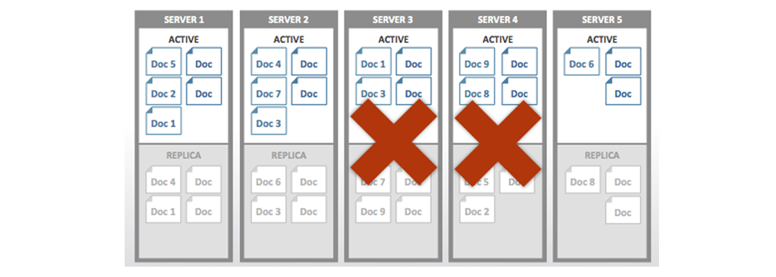
Before you perform a recovery, make sure that your main cluster has an adequate amount of memory and disk space to support the workload as well as the data you recover. This means that even though you can recover data to a cluster with failed nodes, you should investigate what caused the node failures and also make sure your cluster has adequate capacity before you recover data. If you do add nodes be certain to rebalance only after you have For more information about handling node failure in a cluster, see Failing Over Nodes.
When you use cbrecovery it compares the data partitions from a main cluster
with a backup cluster, then sends missing data partitions detected. If it fails,
once you successfully restart cbrecovery, it will do a delta between clusters
again and determine any missing partitions since the failure then resume
restoring these partitions.
Failure Scenarios
Imagine the following happens when you have a four node cluster with one replica. Each node has 256 active and 256 replica vBuckets which total 1024 active and 1024 replica vBuckets:
When one node fails, some active and some replica vBuckets are no longer available in the cluster.
After you fail over this node, the corresponding replica vBuckets on other nodes will be put into an active state. At this point you have a full set of active vBuckets and a partial set of replica vBuckets in the cluster.
A second node fails. More active vBuckets will not be accessible.
You fail over the second node. At this point any missing active vBuckets that do not have corresponding replica vBuckets will be lost.
In this type of scenario you can use cbrecovery to get the missing vBuckets
from your backup cluster. If you have multi-node failure on both your main and
backup clusters you will experience data loss.
Recovery Scenarios for cbrecovery
The following describes some different cluster setups so that you can better understand whether or not this approach will work in your failure scenario:
Multiple Node Failure in Cluster. If multiple nodes fail in a cluster then some vBuckets may be unavailable. In this case if you have already setup XDCR with another cluster, you can recover those unavailable vBuckets from the other cluster.
-
Bucket with Inadequate Replicas.
Single Bucket. In this case where we have only one bucket with zero replicas on all the nodes in a cluster. In this case when a node goes down in the cluster some of the partitions for that node will be unavailable. If we have XDCR set up for this cluster we can recover the missing partitions with
cbrecovery.Multi-Bucket. In this case, nodes in a cluster have multiple buckets and some buckets might have replicas and some do not. In the image below we have a cluster and all nodes have two buckets, Bucket1 and Bucket2. Bucket 1 has replicas but Bucket2 does not. In this case if one of the nodes goes down, since Bucket 1 has replicas, when we failover the node the replicas on other nodes will be activated. But for the bucket with no replicas some partitions will be unavailable and will require
cbrecoveryto recover data. In this same example if multiple nodes fail in the cluster, we need to perform vBucket recovery both buckets since both will have missing partitions.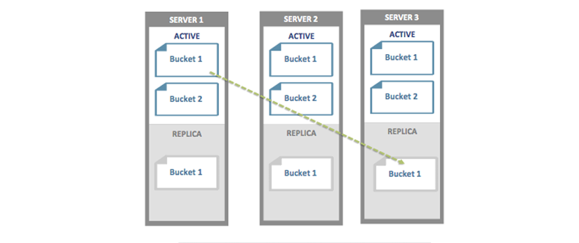
Handling the Recovery
Should you encounter node failure and have unavailable vBuckets, you should follow this process:
-
For each failed node, Click Fail Over under the Server Nodes tab in Web Console. For more information, see Initiating a Node Failover.
After you click Fail Over, under Web Console | Log tab you will see whether data is unavailable and which vBuckets are unavailable. If you do not have enough replicas for the number of failed over nodes, some vBuckets will no longer be available:
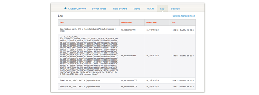
-
Add new functioning nodes to replace the failed nodes.
Do not rebalance after you add new nodes to the cluster. Typically you do this after adding nodes to a cluster, but in this scenario the rebalance will destroy information about the missing vBuckets and you cannot recover them.
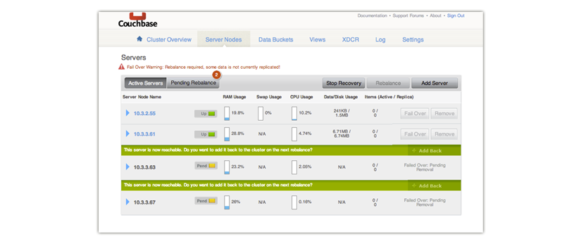
In this example we have two nodes that failed in a three-node cluster and we add a new node 10.3.3.61.
If you are certain your cluster can easily handle the workload and recovered data, you may choose to skip this step. For more instructions on adding nodes, see Adding a Node to a Cluster.
-
Run
cbrecoveryto recover data from your backup cluster. In the Server Panel, a Stop Recovery button appears.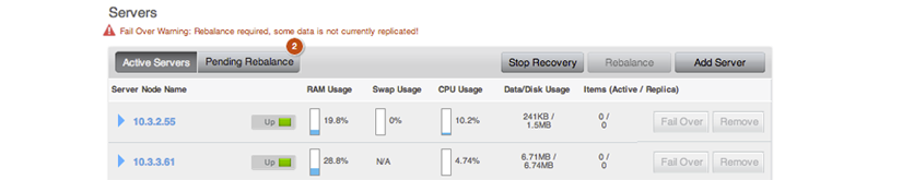
After the recovery completes, this button disappears.
-
Rebalance your cluster. For more information, see Performing a Rebalance.
Once the recovery is done, you can rebalance your cluster, which will recreate replica vBuckets and evenly redistribute them across the cluster.
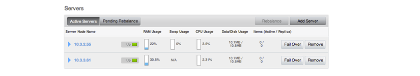
Recovery ‘Dry-Run’
Before you recover vBuckets, you may want to preview a list of buckets no longer available in the cluster. Use this command and options:
shell> ./cbrecovery http://Administrator:password@10.3.3.72:8091 http://Administrator:password@10.3.3.61:8091 -n
Here we provide administrative credentials for the node in the cluster as well
as the option -n. This will return a list of vBuckets in the remote secondary
cluster which are no longer in the your first cluster. If there are any
unavailable buckets in the cluster with failed nodes, you see output as follows:
2013-04-29 18:16:54,384: MainThread Missing vbuckets to be recovered:[{"node": "ns_1@10.3.3.61",
"vbuckets": [513, 514, 515, 516, 517, 518, 519, 520, 521, 522, 523, 524, 525, 526,, 528, 529,
530, 531, 532, 533, 534, 535, 536, 537, 538, 539, 540, 541, 542, 543, 544, 545,, 547, 548,
549, 550, 551, 552, 553, 554, 555, 556, 557, 558, 559, 560, 561, 562, 563, 564, 565, 566, 567,
568, 569, 570, 571, 572,....
Where the vbuckets array contains all the vBuckets that are no longer
available in the cluster. These are the bucket you can recover from the remotes
cluster. To recover the vBuckets:
shell> ./cbrecovery http://Administrator:password@<From_IP>:8091 \
http://Administrator:password@<To_IP>:8091 -B bucket_name
You can run the command on either the cluster with unavailable vBuckets or on
the remote cluster, as long as you provide the hostname, port, and credentials
for remote cluster and the cluster with missing vBuckets in that order. If you
do not provide the parameter -B the tool assumes you will recover unavailable
vBuckets for the default bucket.
Monitoring the Recovery Process
You can monitor the progress of recovery under the Data Buckets tab of Couchbase Web Console:
Click on the Data Buckets tab.
Select the data bucket you are recovering in the Data Buckets drop-down.
-
Click on the Summary drop-down to see more details about this data bucket. You see an increased number in the
itemslevel during recovery:
-
You can also see the number of active vBuckets increase as they are recovered until you reach 1024 vBuckets. Click on the vBucket Resources drop-down:

-
As this tool runs from the command line you can stop it at any time as you would any other command-line tool.
A
Stop Recoverybutton appears in the Servers panels. If you click this button, you will stop the recovery process between clusters. Once the recovery process completes, this button will no longer appear and you will need to rebalance the cluster. If you are in Couchbase Web Console, you can also stop it in this panel: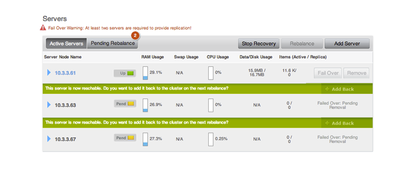
After recovery completes, click on the Server Nodes tab then Rebalance to rebalance your cluster.
When cbrecovery finishes it will output a report in the console:
Recovery : Total | Per sec
batch : 0000 | 14.5
byte : 0000 | 156.0
msg : 0000 | 15.6
4 vbuckets recovered with elapsed time 10.90 seconds
In this report batch is a group of internal operations performed by
cbrecovery, byte indicates the total number of bytes recovered and msg is
the number of documents recovered.
Backup and restore
Backing up your data should be a regular process on your cluster to ensure that you do not lose information in the event of a serious hardware or installation failure.
There are a number of methods for performing a backup:
-
Using
cbbackupThe
cbbackupcommand enables you to back up a single node, single buckets, or the entire cluster into a flexible backup structure that allows for restoring the data into the same, or different, clusters and buckets. All backups can be performed on a live cluster or node. Usingcbbackupis the most flexible and recommended backup tool.For more information, see Backing Up Using cbbackup.
-
Using File Copies
A running or offline cluster can be backed up by copying the files on each of the nodes. Using this method you can only restore to a cluster with an identical configuration.
For more information, see Backing Up Using File Copies.
Due to the active nature of Couchbase Server it is impossible to create a complete in-time backup and snapshot of the entire cluster. Because data is always being updated and modified, it would be impossible to take an accurate snapshot.
For detailed information on the restore processes and options, see Restoring Using cbrestore.
Best Practice
It is a best practice to backup and restore your entire cluster to minimize any inconsistencies in data. Couchbase is always per-item consistent, but does not guarantee total cluster consistency or in-order persistence.
Backing up using cbbackup
The cbbackup tool is a flexible backup command that enables you to backup both
local data and remote nodes and clusters involving different combinations of
your data:
Single bucket on a single node
All the buckets on a single node
Single bucket from an entire cluster
All the buckets from an entire cluster
Backups can be performed either locally, by copying the files directly on a single node, or remotely by connecting to the cluster and then streaming the data from the cluster to your backup location. Backups can be performed either on a live running node or cluster, or on an offline node.
The cbbackup command stores data in a format that allows for easy restoration.
When restoring, using cbrestore, you can restore back to a cluster of any
configuration. The source and destination clusters do not need to match if you
used cbbackup to store the information.
The cbbackup command will copy the data in each course from the source
definition to a destination backup directory. The backup file format is unique
to Couchbase and enables you to restore, all or part of the backed up data when
restoring the information to a cluster. Selection can be made on a key (by
regular expression) or all the data stored in a particular vBucket ID. You can
also select to copy the source data from a bucketname into a bucket of a
different name on the cluster on which you are restoring the data.
The cbbackup command takes the following arguments:
cbbackup [options] [source] [backup_dir]
Note
The cbbackup tool is located within the standard Couchbase command-line
directory. See Command-line Interface.
Be aware that cbbackup does not support external IP addresses. This means that
if you install Couchbase Server with the default IP address, you cannot use an
external hostname to access it. To change the address format into a hostname
format for the server, see Using Hostnames with Couchbase Server.
Where the arguments are as described below:
-
[options]One or more options for the backup process. These are used to configure username and password information for connecting to the cluster, backup type selection, and bucket selection. For a full list of the supported arguments, see cbbackup tool.
The primary options select what will be backed up by
cbbackup, including:-
--single-nodeOnly back up the single node identified by the source specification.
-
--bucket-sourceor-bBackup only the specified bucket name.
-
-
[source]The source for the data, either a local data directory reference, or a remote node/cluster specification:
-
Local Directory ReferenceA local directory specification is defined as a URL using the
couchstore-filesprotocol. For example:couchstore-files:///opt/couchbase/var/lib/couchbase/data/defaultUsing this method you are specifically backing up the specified bucket data on a single node only. To backup an entire bucket data across a cluster, or all the data on a single node, you must use the cluster node specification. This method does not backup the design documents defined within the bucket.
-
cluster nodeA node or node within a cluster, specified as a URL to the node or cluster service. For example:
http://HOST:8091Or for distinction you can use the
couchbaseprotocol prefix:couchbase://HOST:8091The administrator and password can also be combined with both forms of the URL for authentication. If you have named data buckets other than the default bucket which you want to backup, you will need to specify an administrative name and password for the bucket:
couchbase://Administrator:password@HOST:8091The combination of additional options specifies whether the supplied URL refers to the entire cluster, a single node, or a single bucket (node or cluster). The node and cluster can be remote (or local).
This method also backs up the design documents used to define views and indexes.
-
-
-
[backup_dir]The directory where the backup data files will be stored on the node on which the
cbbackupis executed. This must be an absolute, explicit, directory, as the files will be stored directly within the specified directory; no additional directory structure is created to differentiate between the different components of the data backup.The directory that you specify for the backup should either not exist, or exist and be empty with no other files. If the directory does not exist, it will be created, but only if the parent directory already exists.
The backup directory is always created on the local node, even if you are backing up a remote node or cluster. The backup files are stored locally in the backup directory specified.
Backups can take place on a live, running, cluster or node for the IP
Using this basic structure, you can backup a number of different combinations of data from your source cluster. Examples of the different combinations are provided below:
-
Backup all nodes and all buckets
To backup an entire cluster, consisting of all the buckets and all the node data:
> cbbackup http://HOST:8091 /backups/backup-20120501 \ -u Administrator -p password [####################] 100.0% (231726/231718 msgs) bucket: default, msgs transferred… : total | last | per sec batch : 5298 | 5298 | 617.1 byte : 10247683 | 10247683 | 1193705.5 msg : 231726 | 231726 | 26992.7 done [####################] 100.0% (11458/11458 msgs) bucket: loggin, msgs transferred… : total | last | per sec batch : 5943 | 5943 | 15731.0 byte : 11474121 | 11474121 | 30371673.5 msg :84 |84 | 643701.2 doneWhen backing up multiple buckets, a progress report, and summary report for the information transferred will be listed for each bucket backed up. The
msgscount shows the number of documents backed up. Thebyteshows the overall size of the data document data.The source specification in this case is the URL of one of the nodes in the cluster. The backup process will stream data directly from each node in order to create the backup content. The initial node is only used to obtain the cluster topology so that the data can be backed up.
A backup created in this way enables you to choose during restoration how you want to restore the information. You can choose to restore the entire dataset, or a single bucket, or a filtered selection of that information onto a cluster of any size or configuration.
-
Backup all nodes, single bucket
To backup all the data for a single bucket, containing all of the information from the entire cluster:
> cbbackup http://HOST:8091 /backups/backup-20120501 \ -u Administrator -p password \ -b default [####################] 100.0% (231726/231718 msgs) bucket: default, msgs transferred… : total | last | per sec batch : 5294 | 5294 | 617.0 byte : 10247683 | 10247683 | 1194346.7 msg : 231726 | 231726 | 27007.2 doneThe
-boption specifies the name of the bucket that you want to backup. If the bucket is a named bucket you will need to provide administrative name and password for that bucket.To backup an entire cluster, you will need to run the same operation on each bucket within the cluster.
-
Backup single node, all buckets
To backup all of the data stored on a single node across all of the different buckets:
> cbbackup http://HOST:8091 /backups/backup-20120501 \ -u Administrator -p password \ –single-nodeUsing this method, the source specification must specify the node that you want backup. To backup an entire cluster using this method, you should backup each node individually.
-
Backup single node, single bucket
To backup the data from a single bucket on a single node:
> cbbackup http://HOST:8091 /backups/backup-20120501 \ -u Administrator -p password \ –single-node \ -b defaultUsing this method, the source specification must be the node that you want to back up.
-
Backup single node, single bucket; backup files stored on same node
To backup a single node and bucket, with the files stored on the same node as the source data, there are two methods available. One uses a node specification, the other uses a file store specification. Using the node specification:
> ssh USER@HOST remote-> sudo su - couchbase remote-> cbbackup http://127.0.0.1:8091 /mnt/backup-20120501 \ -u Administrator -p password \ –single-node \ -b defaultThis method backups up the cluster data of a single bucket on the local node, storing the backup data in the local filesystem.
Using a file store reference (in place of a node reference) is faster because the data files can be copied directly from the source directory to the backup directory:
> ssh USER@HOST remote-> sudo su - couchbase remote-> cbbackup couchstore-files:///opt/couchbase/var/lib/couchbase/data/default /mnt/backup-20120501To backup the entire cluster using this method, you will need to backup each node, and each bucket, individually.
Choosing the right backup solution will depend on your requirements and your expected method for restoring the data to the cluster.
Filtering keys during backup
The cbbackup command includes support for filtering the keys that are backed
up into the database files you create. This can be useful if you want to
specifically backup a portion of your dataset, or you want to move part of your
dataset to a different bucket.
The specification is in the form of a regular expression, and is performed on
the client-side within the cbbackup tool. For example, to backup information
from a bucket where the keys have a prefix of ‘object’:
> cbbackup http://HOST:8091 /backups/backup-20120501 \
-u Administrator -p password \
-b default \
-k '^object.*'
The above will copy only the keys matching the specified prefix into the backup file. When the data is restored, only those keys that were recorded in the backup file will be restored.
Warning
The regular expression match is performed client side. This means that the
entire bucket contents must be accessed by the cbbackup command and then
discarded if the regular expression does not match.
Key-based regular expressions can also be used when restoring data. You can
backup an entire bucket and restore selected keys during the restore process
using cbrestore. For more information, see Restoring using cbrestore
tool.
Backing up using file copies
You can also backup by using either cbbackup and specifying the local
directory where the data is stored, or by copying the data files directly using
cp, tar or similar.
For example, using cbbackup :
> cbbackup \
couchstore-files:///opt/couchbase/var/lib/couchbase/data/default \
/mnt/backup-20120501
The same backup operation using cp :
> cp -R /opt/couchbase/var/lib/couchbase/data/default \
/mnt/copy-20120501
The limitation of backing up information in this way is that the data can only
be restored to offline nodes in an identical cluster configuration, and where an
identical vbucket map is in operation (you should also copy the config.dat
configuration file from each node.
Restoring using cbrestore
When restoring a backup, you have to select the appropriate restore sequence
based on the type of restore you are performing. The methods available to you
when restoring a cluster are dependent on the method you used when backing up
the cluster. If cbbackup was used to backup the bucket data, you can restore
back to a cluster with the same or different configuration. This is because
cbbackup stores information about the stored bucket data in a format that
enables it to be restored back into a bucket on a new cluster. For all these
scenarios you can use cbrestore. See Restoring using cbrestore
tool.
If the information was backed up using a direct file copy, then you must restore the information back to an identical cluster. See Restoring Using File Copies.
The cbrestore command takes the information that has been backed up via the
cbbackup command and streams the stored data into a cluster. The configuration
of the cluster does not have to match the cluster configuration when the data
was backed up, allowing it to be used when transferring information to a new
cluster or updated or expanded version of the existing cluster in the event of
disaster recovery.
Because the data can be restored flexibly, it allows for a number of different scenarios to be executed on the data that has been backed up:
You want to restore data into a cluster of a different size and configuration.
You want to transfer/restore data into a different bucket on the same or different cluster.
You want to restore a selected portion of the data into a new or different cluster, or the same cluster but a different bucket.
The basic format of the cbrestore command is as follows:
cbrestore [options] [source] [destination]
Where:
-
[options]Options specifying how the information should be restored into the cluster. Common options include:
-
--bucket-sourceSpecify the name of the bucket data to be read from the backup data that will be restored.
-
--bucket-destinationSpecify the name of the bucket the data will be written to. If this option is not specified, the data will be written to a bucket with the same name as the source bucket.
-
--addUse
--addinstead of--setin order to not overwrite existing items in the destination.
For information on all the options available when using
cbrestore, see cbrestore tool -
-
[source]The backup directory specified to
cbbackupwhere the backup data was stored. -
[destination]The REST API URL of a node within the cluster where the information will be restored.
The cbrestore command restores only a single bucket of data at a time. If you
have created a backup of an entire cluster (i.e. all buckets), then you must
restore each bucket individually back to the cluster. All destination buckets
must already exist; cbrestore does not create or configure destination buckets
for you.
For example, to restore a single bucket of data to a cluster:
> cbrestore \
/backups/backup-2012-05-10 \
http://Administrator:password@HOST:8091 \
--bucket-source=XXX
[####################] 100.0% (231726/231726 msgs)
bucket: default, msgs transferred...
: total | last | per sec
batch : 232 | 232 | 33.1
byte : 10247683 | 10247683 | 1462020.7
msg : 231726 | 231726 | 33060.0
done
To restore the bucket data to a different bucket on the cluster:
> cbrestore \
/backups/backup-2012-05-10 \
http://Administrator:password@HOST:8091 \
--bucket-source=XXX \
--bucket-destination=YYY
[####################] 100.0% (231726/231726 msgs)
bucket: default, msgs transferred...
: total | last | per sec
batch : 232 | 232 | 33.1
byte : 10247683 | 10247683 | 1462020.7
msg : 231726 | 231726 | 33060.0
done
The msg count in this case is the number of documents restored back to the
bucket in the cluster.
Filtering keys during restore
The cbrestore command includes support for filtering the keys that are
restored to the database from the files that were created during backup. This is
in addition to the filtering support available during backup (see Filtering
keys during backup ).
The specification is in the form of a regular expression supplied as an option
to the cbrestore command. For example, to restore information to a bucket only
where the keys have a prefix of ‘object’:
> cbrestore /backups/backup-20120501 http://HOST:8091 \
-u Administrator -p password \
-b default \
-k '^object.*'
2013-02-18 10:39:09,476: w0 skipping msg with key: sales_7597_3783_6
...
2013-02-18 10:39:09,476: w0 skipping msg with key: sales_5575_3699_6
2013-02-18 10:39:09,476: w0 skipping msg with key: sales_7597_3840_6
[ ] 0.0% (0/231726 msgs)
bucket: default, msgs transferred...
: total | last | per sec
batch : 1 | 1 | 0.1
byte : 0 | 0 | 0.0
msg : 0 | 0 | 0.0
done
The above will copy only the keys matching the specified prefix into the
default bucket. For each key skipped, an information message will be supplied.
The remaining output shows the records transferred and summary as normal.
Restoring using file copies
To restore the information to the same cluster, with the same configuration, you must shutdown your entire cluster while you restore the data, and then restart the cluster again. You are replacing the entire cluster data and configuration with the backed up version of the data files, and then re-starting the cluster with the saved version of the cluster files.
Important
Make sure that any restoration of files also sets the proper ownership of those files to the couchbase user
When restoring data back in to the same cluster, then the following must be true before proceeding:
The backup and restore must take between cluster using the same version of Couchbase Server.
The cluster must contain the same number of nodes.
Each node must have the IP address or hostname it was configured with when the cluster was backed up.
You must restore all of the
config.datconfiguration files as well as all of the database files to their original locations.
The steps required to complete the restore process are:
Stop the Couchbase Server service on all nodes. For more information, see Server Startup and Shutdown.
On each node, restore the database,
stats.json, and configuration file (config.dat) from your backup copies for each node.Restart the service on each node. For more information, see Server Startup and Shutdown.
Backup and restore between Mac OS X and other platforms
Couchbase Server on Mac OS X uses a different number of configured vBuckets than the Linux and Windows installations. Because of this, backing up from Mac OS X and restoring to Linux or Windows, or vice versa, requires using the built-in Moxi server and the memcached protocol. Moxi will rehash the stored items into the appropriate bucket.
-
Backing up Mac OS X and restoring on Linux/Windows
To backup the data from Mac OS X, you can use the standard
cbbackuptool and options:> cbbackup http://Administrator:password@mac:8091 /macbackup/todayTo restore the data to a Linux/Windows cluster, you must connect to the Moxi port (11211) on one of the nodes within your destination cluster and use the Memcached protocol to restore the data. Moxi will rehash the information and distribute the data to the appropriate node within the cluster. For example:
> cbrestore /macbackup/today memcached://linux:11211 -b default -B defaultIf you have backed up multiple buckets from your Mac, you must restore to each bucket individually.
-
Backing Up Linux/Windows and restoring on Mac OS X
To backup the data from Linux or Windows, you can use the standard
cbbackuptool and options:> cbbackup http://Administrator:password@linux:8091 /linuxbackup/todayTo restore to the Mac OS X node or cluster, you must connect to the Moxi port (11211) and use the Memcached protocol to restore the data. Moxi will rehash the information and distribute the data to the appropriate node within the cluster. For example:
> cbrestore /linuxbackup/today memcached://mac:11211 -b default -B default -
Transferring data directly
You can use
cbtransferto perform the data move directly between Mac OS X and Linux/Windows clusters without creating the backup file, providing you correctly specify the use of the Moxi and Memcached protocol in the destination:> cbtransfer http://linux:8091 memcached://mac:11211 -b default -B default > cbtransfer http://mac:8091 memcached://linux:11211 -b default -B defaultImportant
These transfers will not transfer design documents, since they are using the Memcached protocol
-
Transferring design documents
Because you are restoring data using the Memcached protocol, design documents are not restored. A possible workaround is to modify your backup directory. Using this method, you first delete the document data from the backup directory, and then use the standard restore process. This will restore only the design documents. For example:
> cbbackup http://Administrator:password@linux:8091 /linuxbackup/todayRemove or move the data files from the backup out of the way:
> mv /linuxbackup/today/bucket-default/* /tmpOnly the design document data will remain in the backup directory, you can now restore that information using
cbrestoreas normal:> cbrestore /linuxbackup/today http://mac:8091 -b default -B default
Rebalancing tasks
As you store data into your Couchbase Server cluster, you may need to alter the number of nodes in your cluster to cope with changes in your application load, RAM, disk I/O and networking performance requirements.
Couchbase Server is designed to actively change the number of nodes configured within the cluster to cope with these requirements, all while the cluster is up and running and servicing application requests. The overall process is broken down into two stages; the addition and/or removal of nodes in the cluster, and the
rebalancingof the information across the nodes.The addition and removal process merely configures a new node into the cluster, or marks a node for removal from the cluster. No actual changes are made to the cluster or data when configuring new nodes or removing existing ones.
During the rebalance operation:
-
Using the new Couchbase Server cluster structure, data is moved between the vBuckets on each node from the old structure. This process works by exchanging the data held in vBuckets on each node across the cluster. This has two effects:
Removes the data from machines being removed from the cluster. By totally removing the storage of data on these machines, it allows for each removed node to be taken out of the cluster without affecting the cluster operation.
Adds data and enables new nodes so that they can serve information to clients. By moving active data to the new nodes, they will be made responsible for the moved vBuckets and for servicing client requests.
Rebalancing moves both the data stored in RAM, and the data stored on disk for each bucket, and for each node, within the cluster. The time taken for the move is dependent on the level of activity on the cluster and the amount of stored information.
The cluster remains up, and continues to service and handle client requests. Updates and changes to the stored data during the migration process are tracked and will be updated and migrated with the data that existed when the rebalance was requested.
The current vBucket map, used to identify which nodes in the cluster are responsible for handling client requests, is updated incrementally as each vBucket is moved. The updated vBucket map is communicated to Couchbase client libraries and enabled smart clients (such as Moxi), and allows clients to use the updated structure as the rebalance completes. This ensures that the new structure is used as soon as possible to help spread and even out the load during the rebalance operation.
Because the cluster stays up and active throughout the entire process, clients can continue to store and retrieve information and do not need to be aware that a rebalance operation is taking place.
There are four primary reasons that you perform a rebalance operation:
Adding nodes to expand the size of the cluster.
Removing nodes to reduce the size of the cluster.
Reacting to a failover situation, where you need to bring the cluster back to a healthy state.
You need to temporarily remove one or more nodes to perform a software, operating system or hardware upgrade.
Regardless of the reason for the rebalance, the purpose of the rebalance is migrate the cluster to a healthy state, where the configured nodes, buckets, and replicas match the current state of the cluster.
For information and guidance on choosing how, and when, to rebalance your cluster, read Choosing When to Rebalance. This will provide background information on the typical triggers and indicators that your cluster requires changes to the node configuration, and when a good time to perform the rebalance is required.
Instructions on how to expand and shrink your cluster, and initiate the rebalance operation are provided in Performing a Rebalance.
Once the rebalance operation has been initiated, you should monitor the rebalance operation and progress. You can find information on the statistics and events to monitor using Monitoring a Rebalance.
Common questions about the rebalancing operation are located in Common Rebalancing Questions.
For a deeper background on the rebalancing and how it works, see Rebalance Behind-the-Scenes.
Choosing when to rebalance
Choosing when each of situations applies is not always straightforward. Detailed below is the information you need to choose when, and why, to rebalance your cluster under different scenarios.
Choosing when to expand the size of your cluster
You can increase the size of your cluster by adding more nodes. Adding more nodes increases the available RAM, disk I/O and network bandwidth available to your client applications and helps to spread the load around more machines. There are a few different metrics and statistics that you can use on which to base your decision:
-
Increasing RAM capacity
One of the most important components in a Couchbase Server cluster is the amount of RAM available. RAM not only stores application data and supports the Couchbase Server caching layer, it is also actively used for other operations by the server, and a reduction in the overall available RAM may cause performance problems elsewhere.
There are two common indicators for increasing your RAM capacity within your cluster:
If you see more disk fetches occurring, that means that your application is requesting more and more data from disk that is not available in RAM. Increasing the RAM in a cluster will allow it to store more data and therefore provide better performance to your application.
If you want to add more buckets to your Couchbase Server cluster you may need more RAM to do so. Adding nodes will increase the overall capacity of the system and then you can shrink any existing buckets in order to make room for new ones.
-
Increasing disk I/O throughput
By adding nodes to a Couchbase Server cluster, you will increase the aggregate amount of disk I/O that can be performed across the cluster. This is especially important in high-write environments, but can also be a factor when you need to read large amounts of data from the disk.
-
Increasing disk capacity
You can either add more disk space to your current nodes or add more nodes to add aggregate disk space to the cluster.
-
Increasing network bandwidth
If you see that you are or are close to saturating the network bandwidth of your cluster, this is a very strong indicator of the need for more nodes. More nodes will cause the overall network bandwidth required to be spread out across additional nodes, which will reduce the individual bandwidth of each node.
Choosing when to shrink your cluster
Choosing to shrink a Couchbase cluster is a more subjective decision. It is usually based upon cost considerations, or a change in application requirements not requiring as large a cluster to support the required load.
When choosing whether to shrink a cluster:
You should ensure you have enough capacity in the remaining nodes to support your dataset and application load. Removing nodes may have a significant detrimental effect on your cluster if there are not enough nodes.
You should avoid removing multiple nodes at once if you are trying to determine the ideal cluster size. Instead, remove each node one at a time to understand the impact on the cluster as a whole.
-
You should remove and rebalance a node, rather than using failover. When a node fails and is not coming back to the cluster, the failover functionality will promote its replica vBuckets to become active immediately. If a healthy node is failed over, there might be some data loss for the replication data that was in flight during that operation. Using the remove functionality will ensure that all data is properly replicated and continuously available.
Choosing when to rebalance
Once you decide to add or remove nodes to your Couchbase Server cluster, there are a few things to take into consideration:
If you’re planning on adding and/or removing multiple nodes in a short period of time, it is best to add them all at once and then kick-off the rebalancing operation rather than rebalance after each addition. This will reduce the overall load placed on the system as well as the amount of data that needs to be moved.
Choose a quiet time for adding nodes. While the rebalancing operation is meant to be performed online, it is not a “free” operation and will undoubtedly put increased load on the system as a whole in the form of disk IO, network bandwidth, CPU resources and RAM usage.
Voluntary rebalancing (i.e. not part of a failover situation) should be performed during a period of low usage of the system. Rebalancing is a comparatively resource intensive operation as the data is redistributed around the cluster and you should avoid performing a rebalance during heavy usage periods to avoid having a detrimental affect on overall cluster performance.
Rebalancing requires moving large amounts of data around the cluster. The more RAM that is available will allow the operating system to cache more disk access which will allow it to perform the rebalancing operation much faster. If there is not enough memory in your cluster the rebalancing may be very slow. It is recommended that you don’t wait for your cluster to reach full capacity before adding new nodes and rebalancing.
Rebalancing a cluster
Rebalancing a cluster involves marking nodes to be added or removed from the cluster, and then starting the rebalance operation so that the data is moved around the cluster to reflect the new structure.
Important
Until you complete a rebalance, avoid using the failover functionality since that may result in loss of data that has not yet been replicated.
For information on adding nodes to your cluster, see Adding a Node to a Cluster.
For information on removing nodes to your cluster, see Removing a Node from a Cluster.
In the event of a failover situation, a rebalance is required to bring the cluster back to a healthy state and re-enable the configured replicas. For more information on how to handle a failover situation, see Failing Over Nodes
The Couchbase Admin Web Console will indicate when the cluster requires a rebalance because the structure of the cluster has been changed, either through adding a node, removing a node, or due to a failover. The notification is through the count of the number of servers that require a rebalance. You can see a sample of this in the figure below, here shown on the
Manage Server Nodespage.
To rebalance the cluster, you must initiate the rebalance process, detailed in Performing a Rebalance.
Adding a node to a cluster
There are a number of methods available for adding a node to a cluster. The result is the same in each case, the node is marked to be added to the cluster, but the node is not an active member until you have performed a rebalance operation. The methods are:
-
Web Console — During Installation
When you are performing the Setup of a new Couchbase Server installation (see Initial Server Setup ), you have the option of joining the new node to an existing cluster.
During the first step, you can select the
Join a cluster nowradio button, as shown in the figure below: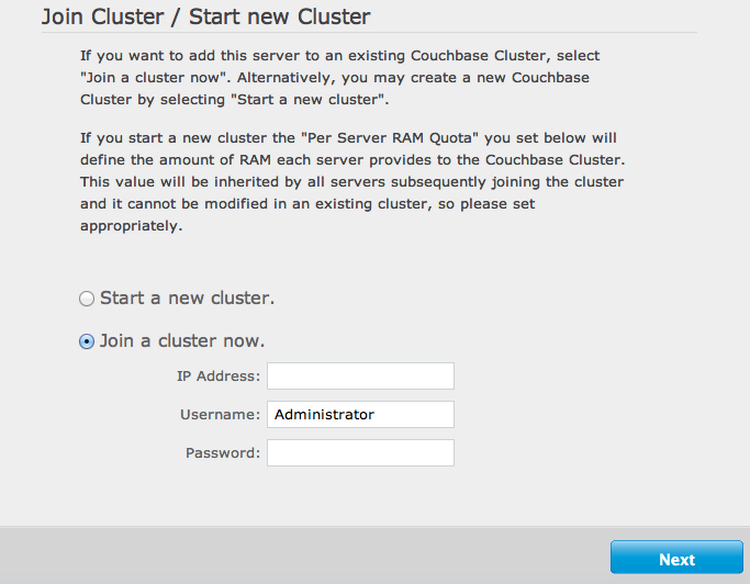
You are prompted for three pieces of information:
-
IP AddressThe IP address of any existing node within the cluster you want to join.
-
UsernameThe username of the administrator of the target cluster.
-
PasswordThe password of the administrator of the target cluster.
The node will be created as a new cluster, but the pending status of the node within the new cluster will be indicated on the Cluster Overview page, as seen in the example below:
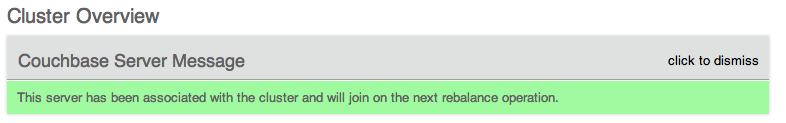
-
-
Web Console — After Installation
You can add a new node to an existing cluster after installation by clicking the
Add Serverbutton within theManage Server Nodesarea of the Admin Console. You can see the button in the figure below.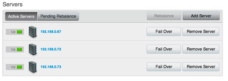
You will be presented with a dialog box, as shown below. Couchbase Server should be installed, and should have been configured as per the normal setup procedures. You can also add a server that has previously been part of this or another cluster using this method. The Couchbase Server must be running.
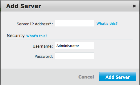
You need to fill in the requested information:
-
Server IP AddressThe IP address of the server that you want to add.
-
UsernameThe username of the administrator of the target node.
-
PasswordThe password of the administrator of the target node.
You will be provided with a warning notifying you that the operation is destructive on the destination server. Any data currently stored on the server will be deleted, and if the server is currently part of another cluster, it will be removed and marked as failed over in that cluster.
Once the information has been entered successfully, the node will be marked as ready to be added to the cluster, and the servers pending rebalance count will be updated.
-
-
Using the REST API
With the REST API, you can add nodes to the cluster by providing the IP address, administrator username and password as part of the data payload. For example, using
curlyou could add a new node:> curl -u cluster-username:cluster-password\ localhost:8091/controller/addNode \ -d "hostname=192.168.0.68&user=node-username&password=node-password"For more information, see Adding a node to a cluster.
-
Using the Command-line interface
You can use the
couchbase-clicommand-line tool to add one or more nodes to an existing cluster. The new nodes must have Couchbase Server installed, and Couchbase Server must be running on each node.To add, run the command:
> couchbase-cli server-add \ –cluster=localhost:8091 \ -u cluster-username -p cluster-password \ –server-add=192.168.0.72:8091 \ –server-add-username=node-username \ –server-add-password=node-passwordWhere:
Parameter Description --clusterThe IP address of a node in the existing cluster. -uThe username for the existing cluster. -pThe password for the existing cluster. --server-addThe IP address of the node to be added to the cluster. --server-add-usernameThe username of the node to be added. --server-add-passwordThe password of the node to be added. If the add process is successful, you will see the following response:
SUCCESS: server-add 192.168.0.72:8091If you receive a failure message, you will be notified of the type of failure.
You can add multiple nodes in one command by supplying multiple
--server-addcommand-line options to the command.
Note
Once a server has been successfully added, the Couchbase Server cluster will indicate that a rebalance is required to complete the operation.
You can cancel the addition of a node to a cluster without having to perform a rebalance operation. Canceling the operation will remove the server from the cluster without having transferred or exchanged any data, since no rebalance operation took place. You can cancel the operation through the web interface.
Removing a node from a cluster
Removing a node marks the node for removal from the cluster and completely disables the node from serving any requests across the cluster. Once removed, a node is no longer part of the cluster in any way and can be switched off, or can be updated or upgraded.
Important
Before you remove a node from the cluster, ensure that you have the capacity within the remaining nodes of your cluster to handle your workload. For more information on the considerations, see Choosing When to Shrink Your Cluster. For the best results, use swap rebalance to swap the node you want to remove out, and swap in a replacement node. For more information on swap rebalance, see Swap Rebalance.
Like adding nodes, there are a number of solutions for removing a node:
-
Web Console
You can remove a node from the cluster from within the
Manage Server Nodessection of the Web Console, as shown in the figure below.To remove a node, click the
Remove Serverbutton next to the node you want to remove. You will be provided with a warning to confirm that you want to remove the node. ClickRemoveto mark the node for removal. -
Using the Command-line
You cannot mark a node for removal from the command-line without also initiating a rebalance operation. The
rebalancecommand accepts one or more--server-addand/or--server-removeoptions. This adds or removes the server from the cluster, and immediately initiates a rebalance operation.For example, to remove a node during a rebalance operation:
> couchbase-cli rebalance –cluster=127.0.0.1:8091 \ -u Administrator -p Password \ –server-remove=192.168.0.73For more information on the rebalance operation, see Performing a Rebalance.
Removing a node does not stop the node from servicing requests. Instead, it only marks the node ready for removal from the cluster. You must perform a rebalance operation to complete the removal process.
Performing a rebalance
Once you have configured the nodes that you want to add or remove from your cluster, you must perform a rebalance operation. This moves the data around the cluster so that the data is distributed across the entire cluster, removing and adding data to different nodes in the process.
If Couchbase Server identifies that a rebalance is required, either through explicit addition or removal, or through a failover, then the cluster is in a
pending rebalancestate. This does not affect the cluster operation, it merely indicates that a rebalance operation is required to move the cluster into its configured state. To start a rebalance:-
Using the Web Console
Within the
Manage Server Nodesarea of the Couchbase Administration Web Console, a cluster pending a rebalance operation will have enabled theRebalancebutton.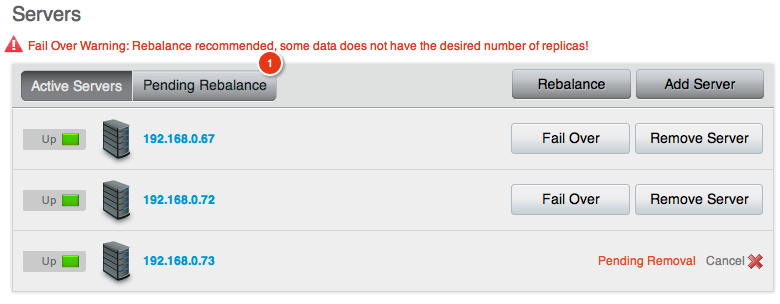
Clicking this button will immediately initiate a rebalance operation. You can monitor the progress of the rebalance operation through the web console.
You can stop a rebalance operation at any time during the process by clicking the
Stop Rebalancebutton. This only stops the rebalance operation, it does not cancel the operation. You should complete the rebalance operation. -
Using the command-line interface
You can initiate a rebalance using the
couchbase-cliand therebalancecommand:> couchbase-cli rebalance -c 127.0.0.1:8091 -u Administrator -p Password INFO: rebalancing … … … … … … … … … … . … … … … … … … … … … … … … . … … … … … … … … … … … … … . … … … … … … … … … … … … … . … … … … … … … … … … … … … . … … … … … … … … … … … … … . … … … . . SUCCESS: rebalanced clusterYou can also use this method to add and remove nodes and initiate the rebalance operation using a single command. You can specify nodes to be added using the
--server-addoption, and nodes to be removed using the--server-remove. You can use multiple options of each type. For example, to add two nodes, and remove two nodes, and immediately initiate a rebalance operation:> couchbase-cli rebalance -c 127.0.0.1:8091 \ -u Administrator -p Password \ –server-add=192.168.0.72 \ –server-add=192.168.0.73 \ –server-remove=192.168.0.70 \ –server-remove=192.168.0.69The command-line provides an active view of the progress and will only return once the rebalance operation has either completed successfully, or in the event of a failure.
You can stop the rebalance operation by using the
stop-rebalancecommand tocouchbase-cli.
The time taken for a rebalance operation depends on the number of servers, quantity of data, cluster performance and any existing cluster activity, and is therefore difficult to accurately predict or estimate.
Throughout any rebalance operation you should monitor the process to ensure that it completes successfully, see Monitoring a Rebalance.
Swap rebalance
Swap Rebalance is an automatic feature that optimizes the movement of data when you are adding and removing the same number of nodes within the same operation. The swap rebalance optimizes the rebalance operation by moving data directly from the nodes being removed to the nodes being added. This is more efficient than standard rebalancing which would normally move data across the entire cluster.
Swap rebalance only occurs if the following are true:
You are removing and adding the same number of nodes during rebalance. For example, if you have marked two nodes to be removed, and added another two nodes to the cluster.
When Couchbase Server identifies that a rebalance is taking place and that there are an even number of nodes being removed and added to the cluster, the swap rebalance method is used to perform the rebalance operation.
Swap rebalance occurs automatically if the number of nodes being added and removed are identical. There is no configuration or selection mechanism to force a swap rebalance. If a swap rebalance cannot take place, then a normal rebalance operation will be used instead.
When a swap rebalance takes place, the rebalance operates as follows:
Data will be moved directly from a node being removed to a node being added on a one-to-one basis. This eliminates the need to restructure the entire vBucket map.
Active vBuckets are moved, one at a time, from a source node to a destination node.
Replica vBuckets are created on the new node and populated with existing data before being activated as the live replica bucket. This ensures that if there is a failure during the rebalance operation, that your replicas are still in place.
For example, if you have a cluster with 20 nodes in it, and configure two nodes (X and Y) to be added, and two nodes to be removed (A and B):
vBuckets from node A will be moved to node X.
vBuckets from node B will be moved to node Y.
The benefits of swap rebalance are:
Reduced rebalance duration. Since the move takes place directly from the nodes being removed to the nodes being added.
Reduced load on the cluster during rebalance.
Reduced network overhead during the rebalance.
Reduced chance of a rebalance failure if a failover occurs during the rebalance operation, since replicas are created in tandem on the new hosts while the old host replicas still remain available.
Because data on the nodes are swapped, rather than performing a full rebalance, the capacity of the cluster remains unchanged during the rebalance operation, helping to ensure performance and failover support.
The behavior of the cluster during a failover and rebalance operation with the swap rebalance functionality affects the following situations:
-
Stopping a rebalance
If rebalance fails, or has been deliberately stopped, the active and replica vBuckets that have been transitioned will be part of the active vBucket map. Any transfers still in progress will be canceled. Restarting the rebalance operation will continue the rebalance from where it left off.
-
Adding back a failed node
When a node has failed, removing it and adding a replacement node, or adding the node back, will be treated as swap rebalance.
Best practice
With swap rebalance functionality, after a node has failed over, either clean up and re-add the failed over node, or add a new node and perform a rebalance as normal. The rebalance will be handled as a swap rebalance which minimize the data movements without affecting the overall capacity of the cluster.
Monitoring a rebalance
You should monitor the system during and immediately after a rebalance operation until you are confident that replication has completed successfully.
A detailed rebalance report is available in the Web Console. As the server moves vBuckets within the cluster, Web Console provides a detailed report. You can view the same statistics in this report via a REST API call, see Getting Rebalance Progress. If you click on the drop-down next to each node, you can view the detailed rebalance status:
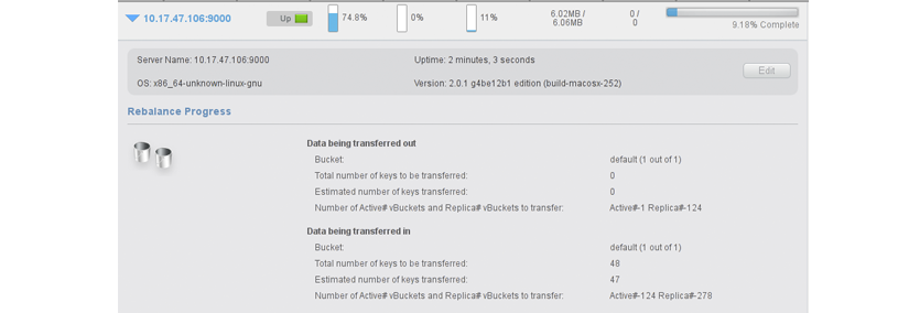
The section
Data being transferred outmeans that a node sends data to other nodes during rebalance. The sectionData being transferred inmeans that a node receives data from other nodes during rebalance. A node can be either a source, a destination, or both a source and destination for data. The progress report displays the following information:Bucket : Name of bucket undergoing rebalance. Number of buckets transferred during rebalance out of total buckets in cluster.
Total number of keys : Total number of keys to be transferred during the rebalance.
Estimated number of keys : Number of keys transferred during rebalance.
Number of Active# vBuckets and Replica# vBuckets : Number of active vBuckets and replica vBuckets to be transferred as part of rebalance.
You can also use
cbstatsto see underlying rebalance statistics:-
Backfilling
The first stage of replication reads all data for a given active vBucket and sends it to the server that is responsible for the replica. This can put increased load on the disk as well as network bandwidth but it is not designed to impact any client activity. You can monitor the progress of this task by watching for ongoing TAP disk fetches. You can also watch
cbstats tap, for example:cbstats <node_IP>:11210 -b bucket_name -p bucket_password tap | grep backfillThis will return a list of TAP backfill processes and whether they are still running (true) or done (false). During the backfill process for a particular tap stream you will see output as follows:
eq_tapq:replication_building_485‘n_1@127.0.0.1’:backfill_completed: false eq_tapq:replication_building_485‘n_1@127.0.0.1’:backfill_start_timestamp: 1371675343 eq_tapq:replication_building_485‘n_1@127.0.0.1’:flags: 85 (ack,backfill,vblist,checkpoints) eq_tapq:replication_building_485‘n_1@127.0.0.1’:pending_backfill: true eq_tapq:replication_building_485‘n_1@127.0.0.1’:pending_disk_backfill: true eq_tapq:replication_building_485‘n_1@127.0.0.1’:queue_backfillremaining: 202When all have completed, you should see the Total Item count (
curr_items_tot) be equal to the number of active items multiplied by replica count. The output you see for a TAP stream after backfill completes is as follows:eq_tapq:replication_building_485‘n_1@127.0.0.1’:backfill_completed: true eq_tapq:replication_building_485‘n_1@127.0.0.1’:backfill_start_timestamp: 1371675343 eq_tapq:replication_building_485‘n_1@127.0.0.1’:flags: 85 (ack,backfill,vblist,checkpoints) eq_tapq:replication_building_485‘n_1@127.0.0.1’:pending_backfill: false eq_tapq:replication_building_485‘n_1@127.0.0.1’:pending_disk_backfill: false eq_tapq:replication_building_485‘n_1@127.0.0.1’:queue_backfillremaining: 0If you are continuously adding data to the system, these values may not correspond exactly at a given instant in time. However you should be able to determine whether there is a significant difference between the two figures.
-
Draining
After the backfill process is complete, all nodes that had replicas materialized on them will then need to persist those items to disk. It is important to continue monitoring the disk write queue and memory usage until the rebalancing operation has been completed, to ensure that your cluster is able to keep up with the write load and required disk I/O.
Common rebalancing questions
Provided below are some common questions and answers for the rebalancing operation.
-
How long will rebalancing take?
Because the rebalancing operation moves data stored in RAM and on disk, and continues while the cluster is still servicing client requests, the time required to perform the rebalancing operation is unique to each cluster. Other factors, such as the size and number of objects, speed of the underlying disks used for storage, and the network bandwidth and capacity will also impact the rebalance speed.
Busy clusters may take a significant amount of time to complete the rebalance operation. Similarly, clusters with a large quantity of data to be moved between nodes on the cluster will also take some time for the operation to complete. A busy cluster with lots of data may take a significant amount of time to fully rebalance.
-
How many nodes can be added or removed?
Functionally there is no limit to the number of nodes that can be added or removed in one operation. However, from a practical level you should be conservative about the numbers of nodes being added or removed at one time.
When expanding your cluster, adding more nodes and performing fewer rebalances is the recommend practice.
When removing nodes, you should take care to ensure that you do not remove too many nodes and significantly reduce the capability and functionality of your cluster.
Remember as well that you can remove nodes, and add nodes, simultaneously. If you are planning on performing a number of addition and removals simultaneously, it is better to add and remove multiple nodes and perform one rebalance, than to perform a rebalance operation with each individual move.
If you are swapping out nodes for servicing, then you can use this method to keep the size and performance of your cluster constant.
-
Will cluster performance be affected during a rebalance?
By design, there should not be any significant impact on the performance of your application. However, it should be obvious that a rebalance operation implies a significant additional load on the nodes in your cluster, particularly the network and disk I/O performance as data is transferred between the nodes.
Ideally, you should perform a rebalance operation during the quiet periods to reduce the impact on your running applications.
-
Can I stop a rebalance operation?
The vBuckets within the cluster are moved individually. This means that you can stop a rebalance operation at any time. Only the vBuckets that have been fully migrated will have been made active. You can re-start the rebalance operation at any time to continue the process. Partially migrated vBuckets are not activated.
The one exception to this rule is when removing nodes from the cluster. Stopping the rebalance cancels their removal. You will need to mark these nodes again for removal before continuing the rebalance operation.
To ensure that the necessary clean up occurs, stopping a rebalance incurs a five minute grace period before the rebalance can be restarted. This ensures that the cluster is in a fixed state before rebalance is requested again.
Rebalance effect on bucket types
The rebalance operation works across the cluster on both Couchbase and
memcachedbuckets, but there are differences in the rebalance operation due to the inherent differences of the two bucket types.For Couchbase buckets:
Data is rebalance across all the nodes in the cluster to match the new configuration.
Updated vBucket map is communicated to clients as each vBucket is successfully moved.
No data is lost, and there are no changes to the caching or availability of individual keys.
For
memcachedbuckets:If new nodes are being added to the cluster, the new node is added to the cluster, and the node is added to the list of nodes supporting the memcached bucket data.
If nodes are being removed from the cluster, the data stored on that node within the memcached bucket will be lost, and the node removed from the available list of nodes.
In either case, the list of nodes handling the bucket data is automatically updated and communicated to the client nodes. Memcached buckets use the Ketama hashing algorithm which is designed to cope with server changes, but the change of server nodes may shift the hashing and invalidate some keys once the rebalance operation has completed.
Rebalance behind-the-scenes
The rebalance process is managed through a specific process called the
orchestrator. This examines the current vBucket map and then combines that information with the node additions and removals in order to create a new vBucket map.The orchestrator starts the process of moving the individual vBuckets from the current vBucket map to the new vBucket structure. The process is only started by the orchestrator - the nodes themselves are responsible for actually performing the movement of data between the nodes. The aim is to make the newly calculated vBucket map match the current situation.
Each vBucket is moved independently, and a number of vBuckets can be migrated simultaneously in parallel between the different nodes in the cluster. On each destination node, a process called
ebucketmigratoris started, which uses the TAP system to request that all the data is transferred for a single vBucket, and that the new vBucket data will become the active vBucket once the migration has been completed.While the vBucket migration process is taking place, clients are still sending data to the existing vBucket. This information is migrated along with the original data that existed before the migration was requested. Once the migration of the all the data has completed, the original vBucket is marked as disabled, and the new vBucket is enabled. This updates the vBucket map, which is communicated back to the connected clients which will now use the new location.
Changing the number of vBucket moves
The number of vBucket moves that occur during the rebalance operation can be modified. The default is one (1), that is, only one vBucket is moved at a time during the rebalance operation.
To change the number of vBucket moves, execute a curl POST command using the following syntax with the
/internalSettingsendpoint andrebalanceMovesPerNodeoption.curl -X POST -u admin:password -d rebalanceMovesPerNode=1 http://HOST:PORT/internalSettingsFor example:
curl -X POST -u Administrator:password -d rebalanceMovesPerNode=14 http://soursop-s11201.sc.couchbase.com:8091/internalSettingsManaging XDCR
Couchbase Server supports cross datacenter replication (XDCR), providing an easy way to replicate data from one cluster to another for disaster recovery as well as better data locality (getting data closer to its users).
Configuring XDCR replications
You configure replications using the
XDCRtab of the Administration Web Console. You configure replication on a bucket basis. If you want to replicate data from all buckets in a cluster, you should individually configure replication for each bucket.Before You Configure XDCR
All nodes within each cluster must be configured to communicate with all the nodes on the destination cluster. XDCR will use any node in a cluster to replicate between the two clusters.
Couchbase Server versions and platforms, must match. For instance if you want to replicate from a Linux-based cluster, you need to do so with another Linux-based cluster.
When XDCR performs replication, it exchanges data between clusters over TCP/IP port 8092; Couchbase Server uses TCP/IP port 8091 to exchange cluster configuration information. If you are communicating with a destination cluster over a dedicated connection or the Internet you should ensure that all the nodes in the destination and source clusters can communicate with each other over ports 8091 and 8092.
Ongoing Replicationsare those replications that are currently configured and operating. You can monitor the current configuration, current status, and the last time a replication process was triggered for each configured replication.Under the XDCR tab you can also configure
Remote Clustersfor XDCR; these are named destination clusters you can select when you configure replication. When you configure XDCR, the destination cluster reference should point to the IP address of one of the nodes in the destination cluster.Warning
Before you set up replication via XDCR, you should be certain that a destination bucket already exists. If this bucket does not exist, replication via XDCR may not find some shards on the destination cluster; this will result in replication of only some data from the source bucket and will significantly delay replication. This would also require you to retry replication multiple times to get a source bucket to be fully replicated to a destination.
Therefore make sure that you check that a destination bucket exists. The recommended approach is to try to read on any key from the bucket. If you receive a 'key not found' error, or the document for the key, the bucket exists and is available to all nodes in a cluster. You can do this via a Couchbase SDK with any node in the cluster. See Couchbase Developer Guide 2.0: Performing Connect, Set and Get.
For more information about creating buckets via the REST API, see Creating and Editing Data Buckets.
Setting source and destination clusters
To create a unidirectional replication (from cluster A to cluster B):
- Check to ensure that a destination bucket exists on the cluster to which you will be replicating. To do so, perform this REST API request:
curl -u Admin:password http://ip.for.destination.cluster:8091/pools/default/buckets-
To set up a destination cluster reference, click the
Create Cluster Referencebutton. You will be prompted to enter a name used to identify this cluster, the IP address, and optionally the administration port number for the remote cluster.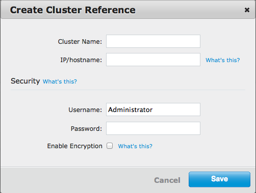
Enter the username and password for the administrator on the destination cluster.
Click Save to store new reference to the destination cluster. This cluster information will now be available when you configure replication for your source cluster.
Creating new replications
After you create references to the source and destination, you can create a replication between the clusters in Couchbase Web Console.
Click
Create Replicationto configure a new XDCR replication. A panel appears where you can configure a new replication from source to destination cluster.In the
Replicate changes fromsection select a from the current cluster that is to be replicated. This is your source bucket.-
In the
Tosection, select a destination cluster and enter a bucket name from the destination cluster: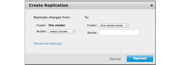
Click the
Replicatebutton to start the replication process.
After you have configured and started replication, the web console will show the current status and list of replications in the
Ongoing Replicationssection: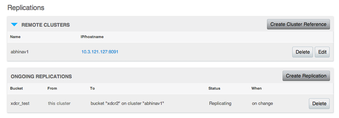
Providing XDCR advanced settings
When you create a new replication, you can also provide internal settings and choose the protocol used for replication at the destination cluster. For earlier versions of Couchbase Server, these internal settings were only available via the REST API, see Changing Internal XDCR Settings.
If you want to change the replication protocol for an existing XDCR replication, you need to delete the replication and then re-create the replication with your preference.
-
In the Create Replication panel, click Advanced settings.
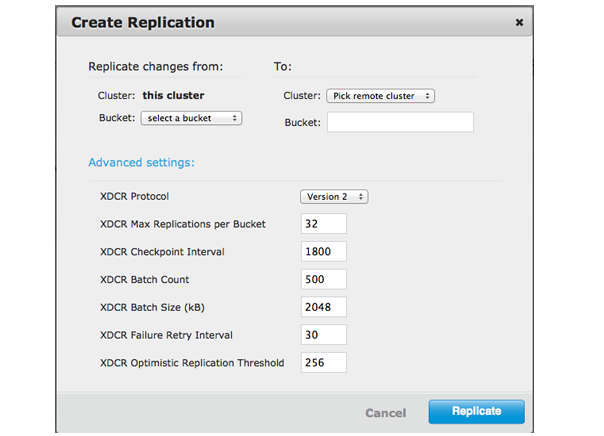
-
Under Advanced settings, choose an XDCR Protocol version.
The XDCR protocol defaults to version 2.
Version 1 uses the REST protocol for replication. This increases XDCR throughput at destination clusters. If you use the Elasticsearch plug-in, which depends on XDCR, choose version 1.
Version 2 uses memcached REST protocol for replication. It is a high-performance mode that directly uses the memcached protocol on destination nodes. Choose version 2 when setting up a new replication with Couchbase Server 2.2 or later.
You can also change this setting via the REST API for XDCR internal settings or the
couchbase-clitool.For more information about XDCR, see XDCR Behavior and Limitations. For more information about Elasticsearch, see Couchbase Elasticsearch Guide.
-
Provide any changes for internal XDCR settings. You can also change these settings plus additional internal settings via the REST API.
How you adjust these variables differs based on what whether you want to perform unidirectional or bidirectional replication between clusters. Other factors for consideration include intensity of read/write operations on your clusters, the rate of disk persistence on your destination cluster, and your system environment. Changing these parameters will impact performance of your clusters as well as XDCR replication performance.
Internal settings that you can update in Web Console include:
-
XDCR Max Replications per BucketMaximum concurrent replications per bucket, 8 to 256. This controls the number of parallel replication streams per node. If you are running your cluster on hardware with high-performance CPUs, you can increase this value to improve replication speed.
-
XDCR Checkpoint IntervalInterval between checkpoints, 60 to 14400 (seconds). Default 1800. At this time interval, batches of data via XDCR replication will be placed in the front of the disk persistence queue. This time interval determines the volume of data that will be replicated via XDCR should replication need to restart. The greater this value, the longer amount of time transpires for XDCR queues to grow. For example, if you set this to 10 minutes and a network error occurs, when XDCR restarts replication, 10 minutes of items will have accrued for replication.
Changing this to a smaller value could impact cluster operations when you have significant amount of write operations on a destination cluster and you are performing bidirectional replication with XDCR. For instance, if you set this to 5 minutes, the incoming batches of data via XDCR replication will take priority in the disk write queue over incoming write workload for a destination cluster. This may result in the problem of having an ever growing disk-write queue on a destination cluster; also items in the disk-write queue that are higher priority than the XDCR items will grow staler/older before they are persisted.
-
XDCR Batch CountDocument batching count, 500 to 10000. Default 500. In general, increasing this value by 2 or 3 times will improve XDCR transmissions rates, since larger batches of data will be sent in the same timed interval. For unidirectional replication from a source to a destination cluster, adjusting this setting by 2 or 3 times will improve overall replication performance as long as persistence to disk is fast enough on the destination cluster. Note however that this can have a negative impact on the destination cluster if you are performing bidirectional replication between two clusters and the destination already handles a significant volume of reads/writes.
-
XDCR Batch Size (KB)Document batching size, 10 to 100000 (KB). Default 2048. In general, increasing this value by 2 or 3 times will improve XDCR transmissions rates, since larger batches of data will be sent in the same timed interval. For unidirectional replication from a source to a destination cluster, adjusting this setting by 2 or 3 times will improve overall replication performance as long as persistence to disk is fast enough on the destination cluster. Note however that this can have a negative impact on the destination cluster if you are performing bidirectional replication between two clusters and the destination already handles a significant volume of reads/writes.
-
XDCR Failure Retry IntervalInterval for restarting failed XDCR, 1 to 300 (seconds). Default 30. If you expect more frequent network or server failures, you may want to set this to a lower value. This is the time that XDCR waits before it attempts to restart replication after a server or network failure.
-
XDCR Optimistic Replication Threshold. This will improve latency for XDCR.This is the compressed document size in bytes. 0 to 20971520 Bytes (20MB). Default is 256 Bytes. XDCR will get metadata for documents larger than this size on a single time before replicating the uncompressed document to a destination cluster. For background information, see ‘Optimistic Replication’ in XDCR.
-
Click Replicate.
After you create the replication or update the setting, you can view or edit them once again by clicking Settings in Outgoing Replications.
Configuring Bidirectional Replication
Replication is unidirectional from one cluster to another. To configure bidirectional replication between two clusters, you need to provide settings for two separate replication streams. One stream replicates changes from Cluster A to Cluster B, another stream replicates changes from Cluster B to Cluster A. To configure a bidirectional replication:
Create a replication from Cluster A to Cluster B on Cluster A.
Create a replication from Cluster B to Cluster A on Cluster B.
You do not need identical topologies for both clusters; you can have a different number of nodes in each cluster, and different RAM and persistence configurations.
You can also create a replication using the REST API instead of Couchbase Web Console. For more information, see Getting a Destination Cluster Reference.
After you create a replication between clusters, you can configure the number of parallel replicators that run per node. The default number of parallel, active streams per node is 32, but you can adjust this. For information on changing the internal configuration settings, see Viewing Internal XDCR Settings.
Monitoring replication status
The following indicate the different areas of the Couchbase Web Console that contains information about replication via XDCR:
- The XDCR tab.
- The outgoing XDCR section under the Data Buckets tab.
The Couchbase Web Console displays replication from the cluster it belongs to. Therefore, when you view the console from a particular cluster, it will display any replications configured, or replications in progress for that particular source cluster. If you want to view information about replications at a destination cluster, you need to open the console at that cluster. Therefore, when you configure bidirectional you should use the web consoles that belong to source and destination clusters to monitor both clusters.
To see statistics on incoming and outgoing replications via XDCR see the following:
Incoming Replications, see Monitoring Incoming XDCR.
Outgoing Replications, see Monitoring Outgoing XDCR.
Any errors that occur during replication appear in the XDCR errors panel. In the example below, we show the errors that occur if replication streams from XDCR will fail due to the missing vBuckets:
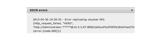
You can tune your XDCR parameters by using the administration REST API. See Viewing Internal XDCR Settings.
Canceling replication
You can cancel replication at any time by clicking
Deletenext to the active replication that is to be canceled.A prompt will confirm the deletion of the configured replication. Once the replication has been stopped, replication will cease on the originating cluster on a document boundary.
Canceled replications that were terminated while the replication was still active will be displayed within the
Past Replicationssection of theReplicationssection of the web console.Upgrading with XDCR
The
xmemreplication mode performs replication on a destination cluster with the memcached protocol. This is the default mode for Couchbase Server replications. Thecapimode performs replications over a REST protocol.-
xmem- only 2.2 servers and above support it. -
capi- both 2.2 and pre-2.2 servers support it.
The following prerequisites need to be considered in order to prevent data loss during replication:
- Network port 11210 needs to be open between nodes for ‘xmem’ mode of replication to work.
- In general, delete the replication, complete the upgrade, then recreate the replication.
- When upgrading Couchbase Server, make sure that both the source and destination clusters support the desired replication mode.
- To use XDCR data encryption with Secure Socket Layer (SSL), all nodes must be upgraded to at least Couchbase Server 2.5 Enterprise Edition.
Consider the following upgrade scenarios:
- Both source and destination clusters are pre-2.2 and both are upgrading to pre-2.2 versions. This scenario is supported since both clusters use
capi. - Both source and destination clusters are pre-2.2 and the destination is upgrading to 2.2. This is a safe upgrade path since the source cluster communicates via
capito the destination. - The source cluster is upgrading to 2.2 or higher and the destination is pre-2.2. This is not a safe upgrade path because the destination cannot receive replication via
xmem. This results in incorrect data replication and failures in conflict resolution. For this scenario, upgrade both source and destination clusters to 2.2 or higher. - Both source and destination clusters are upgrading from pre-2.2 to 2.2. This is not a safe upgrade path because the cluster upgrades are not synchronized. If the source upgrade completes prior to destination upgrade, incorrect data replication and failures in conflict resolution may occur. For this scenario:
- Delete all XDCR replications on your source cluster.
- Upgrade the source cluster to 2.2 or higher.
- Upgrade the destination cluster to 2.2 or higher.
- Re-create the XDCR replications using Version 2 for the XDCR protocol. Version 2 is
xmemreplication.
Alternatively:
- Allow the rebalance upgrade to complete.
- Delete the Version 1 (
capi) XDCR protocol replications. - Create Version 2 (
xmem) XDCR protocol replications.
- The source cluster is upgrading from pre–2.2 to 2.2 or higher and the destination cluster is Elastic Search. Since the source cluster must use capi for replication:
- Delete all XDCR replications on your source cluster.
- Upgrade the source cluster to 2.2 or higher.
- Re-create the XDCR replications using Version 1 for the XDCR protocol. Version 1 is
capireplication.
- Both source and destination clusters are upgraded from pre-2.2 to 2.5 or higher. This is not a safe upgrade path because the cluster upgrades are not synchronized. If the source upgrade completes prior to destination upgrade, incorrect data replication and failures in conflict resolution may occur..
- Delete all XDCR replications on your source cluster.
- Upgrade the source cluster to 2.5 or higher.
- Upgrade the destination cluster to 2.5 or higher.
- Re-create the XDCR replications using Version 2 for the XDCR protocol. Version 2 is
xmemreplication.
Conflict resolution in XDCR
XDCR automatically performs conflict resolution for different document versions on source and destination clusters. The algorithm is designed to consistently select the same document on either a source or destination cluster. For each stored document, XDCR perform checks of metadata to resolve conflicts. It checks the following:
Numerical sequence, which is incremented on each mutation
CAS value
Document flags
Expiration (TTL) value
If a document does not have the highest revision number, changes to this document will not be stored or replicated; instead the document with the highest score will take precedence on both clusters. Conflict resolution is automatic and does not require any manual correction or selection of documents.
By default XDCR fetches metadata twice from every document before it replicates the document at a destination cluster. XDCR fetches metadata on the source cluster and looks at the number of revisions for a document. It compares this number with the number of revisions on the destination cluster and the document with more revisions is considered the ‘winner.’
If XDCR determines a document from a source cluster will win conflict resolution, it puts the document into the replication queue. If the document will lose conflict resolution because it has a lower number of mutations, XDCR will not put it into the replication queue. Once the document reaches the destination, this cluster will request metadata once again to confirm the document on the destination has not changed since the initial check. If the document from the source cluster is still the ‘winner’ it will be persisted onto disk at the destination. The destination cluster will discard the document version with the lowest number of mutations.
The key point is that the number of document mutations is the main factor that determines whether XDCR keeps a document version or not. This means that the document that has the most recent mutation may not be necessarily the one that wins conflict resolution. If both documents have the same number of mutations, XDCR selects a winner based on other document metadata. Precisely determining which document is the most recently changed is often difficult in a distributed system. The algorithm Couchbase Server uses does ensure that each cluster can independently reach a consistent decision on which document wins.
‘Optimistic replication’ in XDCR
XDCR can be tuned the performance of XDCR with the
xdcrOptimisticReplicationThresholdparameter. By default, XDCR gets metadata twice for documents over 256 bytes before it performs conflict resolution for at a destination cluster. If the document fails conflict resolution it will be discarded at the destination cluster.When a document is smaller than the number of bytes provided as this parameter, XDCR immediately puts it into the replication queue without getting metadata on the source cluster. If the document is deleted on a source cluster, XDCR will no longer fetch metadata for the document before it sends this update to a destination cluster. Once a document reaches the destination cluster, XDCR will fetch the metadata and perform conflict resolution between documents. If the document ‘loses’ conflict resolution, Couchbase Server discards it on the destination cluster and keeps the version on the destination. This new feature improves replication latency, particularly when you replicate small documents.
There are tradeoffs when you change this setting. If you set this low relative to document size, XDCR will frequently check metadata. This will increase latency during replication, it also means that it will get metadata before it puts a document into the replication queue, and will get it again for the destination to perform conflict resolution. The advantage is that you do not waste network bandwidth since XDCR will send less documents that will ‘lose.’
If you set this very high relative to document size, XDCR will fetch less metadata which will improve latency during replication. This also means that you will increase the rate at which XDCR puts items immediately into the replication queue which can potentially overwhelm your network, especially if you set a high number of parallel replicators. This may increase the number of documents sent by XDCR which ultimately ‘lose’ conflicts at the destination which wastes network bandwidth.
Note: XDCR does not fetch metadata for documents that are deleted.
Changing the Document Threshold
You can change this setting with the REST API as one of the internal settings for XDCR. For more information, see Changing Internal XDCR Settings.
Monitoring ‘Optimistic Replication"
The easiest way you can monitor the impact of this setting is in Couchbase Web Console. On the Data Buckets tab under Incoming XDCR Operations, you can compare
metadata reads per sectosets per sec: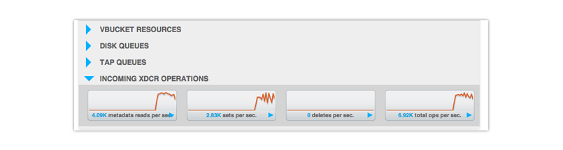
If you set a low threshold relative to document size,
metadata reads per secwill be roughly twice the value ofsets per sec. If you set a high threshold relative to document size, this will virtually eliminate the first fetch of metadata and thereforemetadata reads per secwill roughly equalsets per secThe other option is to check the log files for XDCR, which you can find in
/opt/couchbase/var/lib/couchbase/logson the nodes for a source bucket. The log files following the naming conventionxdcr.1,xdcr.2and so on. In the logs you will see a series of entries as follows:out of all 11 docs, number of small docs (including dels: 2) is 4, number of big docs is 7, threshold is 256 bytes, after conflict resolution at target ("http://Administrator:asdasd@127.0.0.1:9501/default%2f3%3ba19c9d4e733a97fa7cb38daa4113d034/"), out of all big 7 docs the number of docs we need to replicate is: 5; total # of docs to be replicated is: 9, total latency: 142 msThe first line means that 4 documents are under the threshold and XDCR checked metadata twice for all 7 documents and replicated 5 larger documents and 4 smaller documents. The amount of time to check and replicate all 11 documents was 142 milliseconds. For more information about XDCR, see Cross Datacenter Replication (XDCR).
Changing XDCR settings
Besides Couchbase Web Console, you can use several Couchbase REST API endpoints to modify XDCRsettings. Some of these settings are references used in XDCR and some of these settings will change XDCR behavior or performance:
Viewing, setting and removing destination cluster references, can be found in Getting a Destination Cluster Reference, Creating a Destination Cluster Reference and Deleting a Destination Cluster Reference.
Creating and removing a replication via REST can be found in Creating a Destination Cluster Reference and Deleting a Destination Cluster Reference.
Concurrent replications, which is the number of concurrent replications per Couchbase Server instance. See Viewing Internal XDCR Settings.
‘Optimistic Replication.’ For more information about ‘optimistic replication’, see ‘Optimistic Replication’ in XDCR.
For the XDCR retry interval you can provide an environment variable or make a PUT request. By default if XDCR is unable to replicate for any reason like network failures, it will stop and try to reach the remote cluster every 30 seconds if the network is back, XDCR will resume replicating. You can change this default behavior by changing an environment variable or by changing the server parameter
xdcr_failure_restart_intervalwith a PUT request:Note that if you are using XDCR on multiple nodes in cluster and you want to change this setting throughout the cluster, you will need to perform this operation on every node in the cluster.
- By an environment variable:
export XDCR_FAILURE_RESTART_INTERVAL=60- By server setting:
curl -X POST http://Administrator:You can put the system environment variable in a system configuration file on your nodes. When the server restarts, it will load this parameter. If you set both the environment variable and the server parameter, the value for the environment parameter will supersede.
Securing data communication
When configuring XDCR across multiple clusters over public networks, the data is sent unencrypted across the public interface channel. To ensure security for the replicated information you will need to configure a suitable VPN gateway between the two datacenters that will encrypt the data between each route between datacenters.
Within dedicated datacenters being used for Couchbase Server deployments, you can configure a point to point VPN connection using a static route between the two clusters:
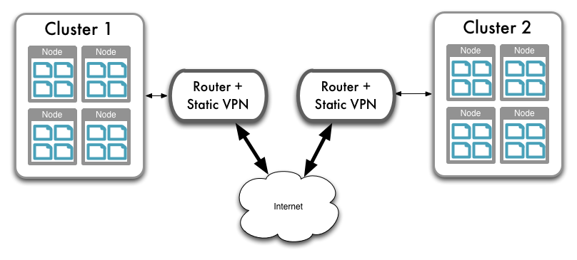
When using Amazon EC2 or other cloud deployment solutions, particularly when using different EC2 zones, there is no built-in VPN support between the different EC2 regional zones. However, there is VPN client support for your cluster within EC2 and Amazon VPC to allow communication to a dedicated VPN solution. For more information, see Amazon Virtual Private Cloud FAQs for a list of supported VPNs.
To support cluster to cluster VPN connectivity within EC2 you will need to configure a multi-point BGP VPN solution that can route multiple VPN connections. You can then route the VPN connection from one EC2 cluster and region to the third-party BGP VPN router, and the VPN connection from the other region, using the BGP gateway to route between the two VPN connections.
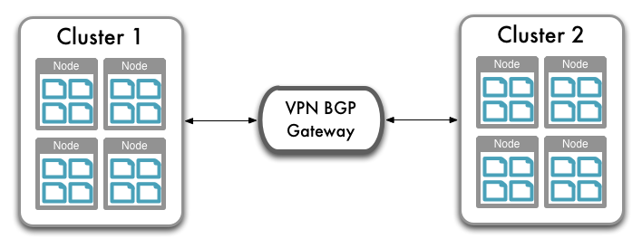
Configuration of these VPN routes and systems is dependent on your VPN solution.
For additional security, you should configure your security groups to allow traffic only on the required ports between the IP addresses for each cluster. To configure security groups, you will need to specify the inbound port and IP address range. You will also need to ensure that the security also includes the right port and IP addresses for the remainder of your cluster to allow communication between the nodes within the cluster.
You must ensure when configuring your VPN connection that you route and secure all the ports in use by the XDCR communication protocol, ports 8091 and 8092 on every node within the cluster at each destination.
Managing XDCR data encryption
The cross data center (XDCR) data security feature (Enterprise Edition only) provides secure cross data center replication using Secure Socket Layer (SSL) data encryption. The data replicated between clusters can be encrypted in both uni-directional and bi-directional replications.
XDCR data encryption prerequisites
- Couchbase servers on both source and destination clusters must have Couchbase 2.5 Enterprise Edition and above installed.
- The source cluster must use the destination cluster’s certificate. The certificate is a self-signed certificate used by SSL to initiate secure sessions.
- The reserved ports for XDCR data encryption must be available.
Note
The certificate is an internal self-signed certificate used by SSL to initiate secure sessions.
With XDCR data encryption, the following ports are reserved:
Port Description 11214 Incoming SSL Proxy 11215 Internal Outgoing SSL Proxy 18091 Internal REST HTTPS for SSL 18092 Internal CAPI HTTPS for SSL Important
Ensure that the Secure Socket Layer (SSL) reserved ports are available prior to using XDCR data encryption. Otherwise, XDCR data encryption is unavailable.
To enable XDCR data security
To enable XDCR data security using SSL and create replication:
- On the destination cluster, navigate to Settings > Cluster and copy the certificate.
- (Optional) To regenerate the existing destination certificate, click Regenerate before copying.
- On the source cluster, select the XDCR tab.
- On the Remote Clusters panel, click Create Cluster Reference to verify or create the cluster reference.
- Select the Enable Encryption box and paste the certificate in the provided area and click Save.
- On the Ongoing Replications panel, click Create Replication, provide the cluster and bucket information, and click Replicate.
To change XDCR data encryption
In some situations (such as updating SSL data security), the SSL certificate is regenerated and the XDCR data encryption is updated. To change XDCR data encryption:
- On the destination cluster, navigate to Settings > Cluster.
- Click Regenerate and copy the certificate.
- On the source cluster, select the XDCR tab.
- On the Remote Clusters panel, for the destination cluster, click Edit.
- Paste the regenerated certificate in the provided area and click Save.
Anytime a destination cluster’s certificate is regenerated, the corresponding source cluster(s) must be updated with the regenerated certificate.
For example, if source clusters A, B, and C use XDCR data encryption to replicate to destination cluster D, each of the source clusters must be updated whenever the certificate on the destination cluster D is regenerated (changed).
Important
If a destination cluster's certificate is regenerated and the source cluster(s) are not updated with the new certificate, replication stops.
SSL certificate
The following is an example of an SSL certificate and where the certificate is obtained on the cluster.
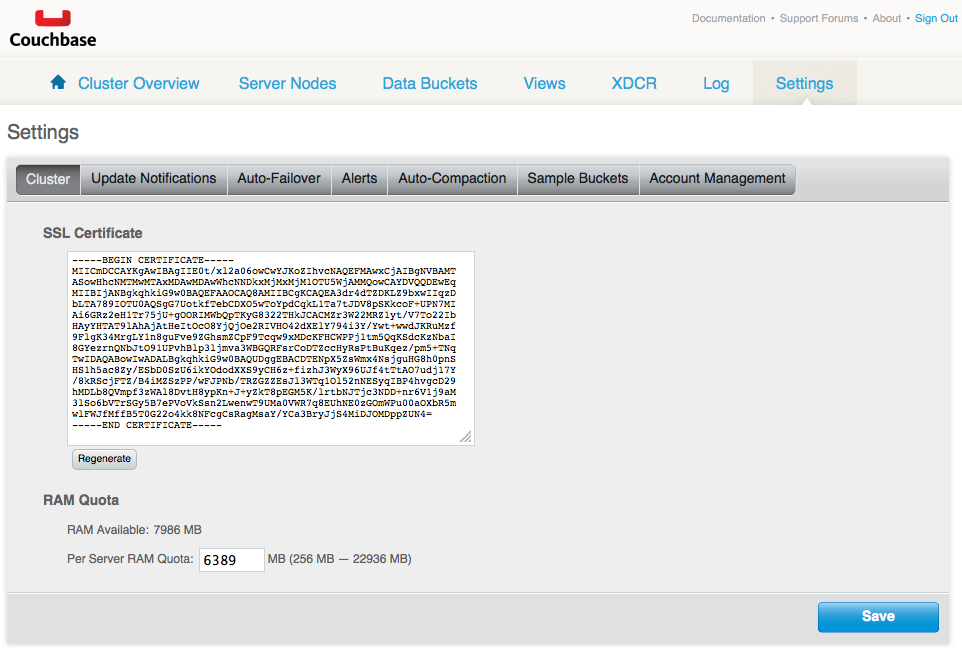
Create Cluster Reference
The following is an example of the Create Cluster Reference pop-up.
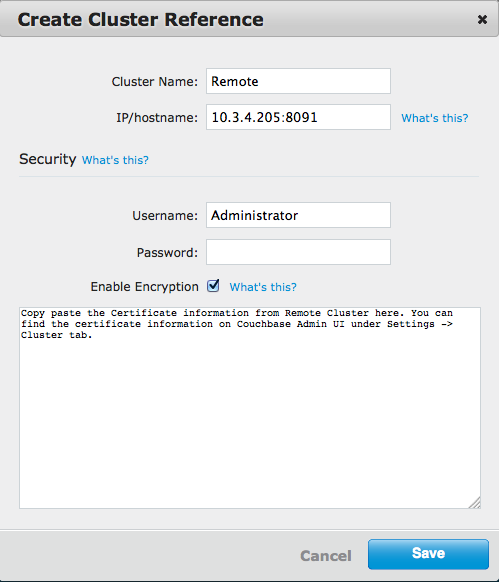
XDCR data security error messages
When creating the cluster reference, if the SSL certificates are not the same on the destination and source clusters, the following error message displays:
Attention - Got certificate mismatch while trying to send https request to HOST:18091If the SSL certificates become mismatched (for example, if the certificate on the destination cluster is regenerated and the source cluster is not updated with the new certificate), vBucket replication stops and the following error message displays:
Error replicating vbucket <bucketNumber>. Please see logs for details.Using XDCR in cloud deployments
If you want to use XDCR within a cloud deployment to replicate between two or more clusters that are deployed in the cloud, there are some additional configuration requirements:
-
Use a public DNS names and public IP addresses for nodes in your clusters.
Cloud services support the use of a public IP address to allow communication to the nodes within the cluster. Within the cloud deployment environment, the public IP address will resolve internally within the cluster, but allow external communication. In Amazon EC2, for example, ensure that you have enabled the public interface in your instance configuration, that the security parameters allow communication to the required ports, and that public DNS record exposed by Amazon is used as the reference name.
You should configure the cluster with a fixed IP address and the public DNS name according to the information in Handling Changes in IP Addresses.
-
Use a DNS service to identify or register a CNAME that points to the public DNS address of each node within the cluster. This will allow you to configure XDCR to use the CNAME to a node in the cluster. The CNAME will be constant, even though the underlying public DNS address may change within the cloud service.
The CNAME record entry can then be used as the destination IP address when configuring replication between the clusters using XDCR. If a transient failure causes the public DNS address for a given cluster node to change, update the CNAME to point to the updated public DNS address provided by the cloud service.
By updating the CNAME records, replication should be able to persist over a public, internet- based connection, even though the individual IP of different nodes within each cluster configured in XDCR.
For additional security, you should configure your security groups to allow traffic only on the required ports between the IP addresses for each cluster. To configure security groups, you will need to specify the inbound port and IP address range. You will also need to ensure that the security also includes the right port and IP addresses for the remainder of your cluster to allow communication between the nodes within the cluster.
For more information about reserved Couchbase ports, see Network ports in Getting started. For more information in general about using Couchbase Server in the cloud, see Using Couchbase in the Cloud.
Managing Rack Awareness
The Rack Awareness feature (Enterprise Edition) allows logical groupings of servers on a cluster where each server group physically belongs to a rack or availability zone. This feature provides the ability to specify that active and corresponding replica partitions be created on servers that are part of a separate rack or zone.
This section describes how to manage server groups through the Web Console. See also, the couchbase-cli, Managing Rack Awareness CLI and Rack Awareness REST API, managing servers and server groups. By default, when a Couchbase cluster is initialized, Group 1 is created.
Rack Awareness prerequisites
To implement Rack Awareness, all servers in the cluster must be upgraded to Couchbase 2.5 Enterprise Edition.
- Configure at least two server groups.
- Configure all of the servers to use server groups.
- Configure each server group to have the same number of servers (recommended).
Rack Awareness Web Console
The servers and server groups are displayed from the Server Nodes tab:

The server groups are edited and created by clicking on Server Groups:
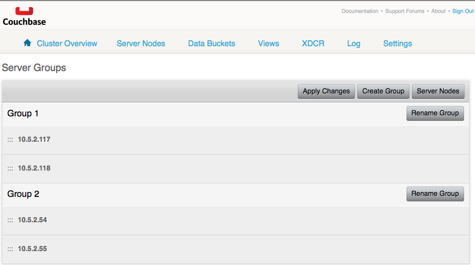
Creating server groups
To create a server group:
- From the Server Nodes tab, click Server Groups.
- Click Create Group and provide a group name to the Add Group pop-up.
- Click Create.
Renaming server groups
To change a server group’s name:
- From the Server Nodes tab, click Server Groups.
- Click Edit Group.
- Change the group name and Save.
Deleting server groups
To delete a server group, first remove all:
- From the Server Nodes tab, click Remove to remove nodes from the server group.
- From the Server Nodes tab, click Server Groups.
- Click on “This group is empty, click to delete.” which is displayed if the server group is empty.
- Click Delete from the Removing pop-up.
Adding servers to server groups
To add a server:
- From the Server Nodes tab, click Add Server.
- Provide the Server IP Address, select a server group from the drop down menu, and provide the administrator username and password for the server being added.
- Click Add Server.
- From the Server Nodes tab, click Rebalance.
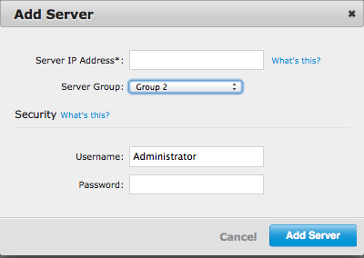
Removing servers from server groups
To remove a server from a server group:
- From the Server Nodes tab, click Remove for the server that you want to delete.
- Click Remove from the confirmation pop-up.
- From the Server Nodes tab, click Rebalance.
Moving servers between server groups
To move a server from one group to another:
- From the Server Nodes tab, Click Server Groups.
- Drag and drop the server from one group to another.
- Click Apply Changes.
- From the Server Nodes tab, click Rebalance.

Changing the configured disk path
You cannot change the disk path where the data and index files are stored on a running server. To change the disk path, the node must be removed from the cluster, configured with the new path, and added back to the cluster.
The quickest and easiest method is to provision a new node with the correct disk path configured, and then use swap rebalance to add the new node in while taking the old node out. For more information, see Swap Rebalance.
To change the disk path of the existing node, the recommended sequence is:
Remove the node where you want to change the disk path from the cluster. For more information, see Removing a Node from a Cluster. To ensure the performance of your cluster is not reduced, perform a swap rebalance with a new node (see Swap Rebalance ).
Perform a rebalance operation, see Performing a Rebalance.
-
Configure the new disk path, either by using the REST API (see Configuring Index Path for a Node ), using the command-line (see cluster initialization for more information).
Alternatively, connect to the Web UI of the new node, and follow the setup process to configure the disk path (see Initial Server Setup.
Add the node back to the cluster, see Adding a Node to a Cluster.
The above process changes the disk path only on the node that was removed from the cluster. To change the disk path on multiple nodes, swap out each node and change the disk path individually.
Rack Awareness
The Rack Awareness feature allows logical groupings of servers on a cluster where each server group physically belongs to a rack or availability zone. This feature provides the ability to specify that active and corresponding replica partitions be created on servers that are part of a separate rack or zone. To enable Rack Awareness, all servers in a cluster must be upgraded to Couchbase Server Enterprise Edition to use the Rack Awareness feature.
For more information, see Managing Rack Awareness.
Note
The Rack Awareness feature with its server group capability is an Enterprise Edition feature.
Definition list:
- Cluster
- Collection of one or more servers or instances of Couchbase Server that are configured as a logical cluster.
- Server (node)
- A single instance of the Couchbase Server software running on a machine, whether a physical machine, virtual machine, EC2 instance or other environment.
- Server group
- Logical group of servers in a cluster.
- Rack
- Physical rack where servers in a server group are located.
- Availability Zone or Region
- Cloud servers hosted in locations that are composed of regions and availability zones. Each region is a separate geographic area. Each region has multiple, isolated locations known as availability zones.
To enable Rack Awareness
- Configure at least two server groups.
- Configure all of the servers to use server groups.
- Configure each server group to have the same number of servers (recommended).
To improve data availability, configure servers into groups where all of the servers in a server group are in a single rack. With more than one rack, replica partitions of a group are distributed among servers in other server groups. In the event that a whole rack goes down, since the replica partitions are on separate racks, data is available.
Important
Couchbase does not automatically failover a server group. Auto-failover only fails over one (1) node. Thereafter, the number of auto failover nodes can be reset to zero (0). If a server group is down, the nodes can be manually failed over.
Replica and replication with server groups
By design, Couchbase Server evenly distributes data of active and replica vBuckets across the cluster for cluster performance and redundancy purposes.
With Rack Awareness, server partitions are laid out so the replica partitions for servers in one server group are distributed in servers for a second group and vice versa. If one of the servers becomes unavailable or if an entire rack goes down, data is retained since the replicas are available on the second server group.
Cluster management with server groups
Rack Awareness feature evenly distributes replica vBuckets from one server group to another server group to provide redundancy and data availability. The rebalance operation evenly distributes the replica vBuckets from one server group to another server group across the cluster. If an imbalance occurs where there is an unequal number of servers in one server group, the rebalance operation performs a “best effort” of evenly distributing the replica vBuckets across the cluster.
Implementation of replica vBuckets
The following example shows how Rack Awareness functionality implements replica vBuckets to provide redundancy. In this example, there are two (2) server groups in the cluster and four (4) servers in each server group. Since there is equal number of servers in each server group, the cluster is balanced which guarantees that replica vBuckets for one server group are on a different server group.
The following diagram shows a cluster of servers on two racks, Rack #1 and Rack #2, where each rack has a group of four (4) servers.
- Group 1 has Servers 1, 2, 3, and 4.
- Group 1 servers have their active vBuckets and replica vBuckets from Group 2.
- Group 2 has Servers 5, 6, 7, and 8.
- Group 2 servers have their active vBuckets and replica vBuckets from Group 1.
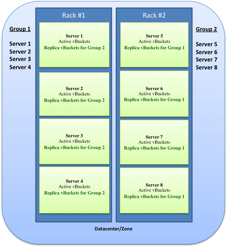
Scenario - Adding a server
The following scenario shows how Rack Awareness functionality implements replica vBuckets when an imbalance is caused by an additional server being added to one server group. In this example, an additional server (Server 9) is added to a server group (Group 1). An imbalance occurs because one server group has more servers than the other server group. In this case, the rebalance operation performs a “best effort” of evenly distributing the replica vBuckets of the additional server across the nodes on all the racks in the cluster.
The following diagram shows a cluster of servers on two racks, Rack #1 and Rack #2, where one rack has a group of five (5) servers and the other rack has a group of four (4) servers.
- Group 1 has Servers 1, 2, 3, 4, and 9
- Group 1 servers have their active vBuckets and replica vBuckets from Group 2.
- Group 1 Servers 1 - 4 also has replica vBuckets for Server 9.
- Group 2 has Servers 5, 6, 7, and 8.
- Group 2 servers have their active vBuckets and replica vBuckets from Group 1 including the replica vBuckets from Server 9 in Group 1.
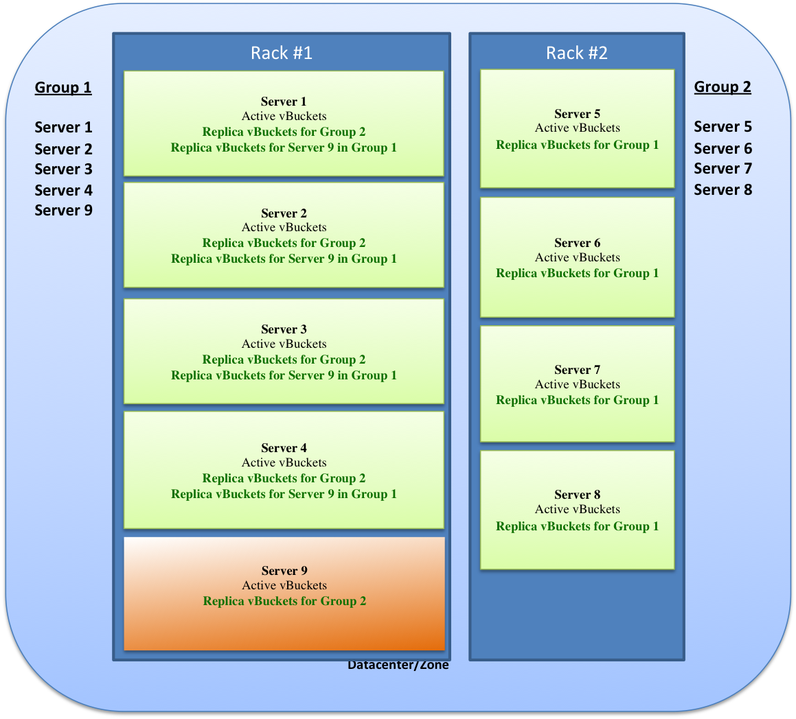
Scenario - Removing a server or server unavailable
The following scenario shows how Rack Awareness functionality implements replica vBuckets when an imbalance is caused by a server being removed or unavailable in a server group. In this example, a server (Server 2) is unavailable to a server group (Group 1). An imbalance occurs because one server group has fewer servers than the other server group. In this case, if the rebalance operation is performed, a “best effort” of evenly distributing the replica vBuckets across the cluster occurs.
Note
If the cluster becomes imbalanced, add servers to balance the cluster. For optimal Rack Awareness functionality, a balanced cluster is recommended.
If there is only one server or only one server group, default behavior is automatically implemented, that is, Rack Awareness functionality is disabled.
The following diagram shows the loss of a server resulting in an imbalance. In this case, Server 2 (from Group 1, Rack #1) becomes unavailable. The replica vBuckets for Server 2 in Group 2, Rack #2 become enabled and rebalancing occurs.
- Group 1 has Servers 1, 2, 3, and 4
- Group 1 servers have their active vBuckets and replica vBuckets from Group 2.
- Group 1 Server 2 becomes unavailable.
- Group 2 has Servers 5, 6, 7, and 8.
- Group 2 servers have their active vBuckets and replica vBuckets from Group 1.
- Group 2 server activates the replica vBuckets for Server 2 in Group 1.
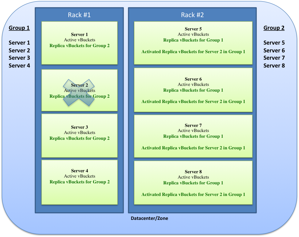
Cross Datacenter Replication (XDCR)
Couchbase Server supports cross datacenter replication (XDCR), providing an easy way to replicate data from one cluster to another for disaster recovery as well as better data locality (getting data closer to its users).
Couchbase Server provides support for both intra-cluster replication and cross datacenter replication (XDCR). Intra-cluster replication is the process of replicating data on multiple servers within a cluster in order to provide data redundancy should one or more servers crash. Data in Couchbase Server is distributed uniformly across all the servers in a cluster, with each server holding active and replica documents. When a new document is added to Couchbase Server, in addition to being persisted, it is also replicated to other servers within the cluster (this is configurable up to three replicas). If a server goes down, failover promotes replica data to active:
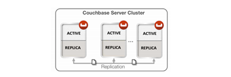
Cross datacenter replication in Couchbase Server involves replicating active data to multiple, geographically diverse datacenters either for disaster recovery or to bring data closer to its users for faster data access, as shown in below:
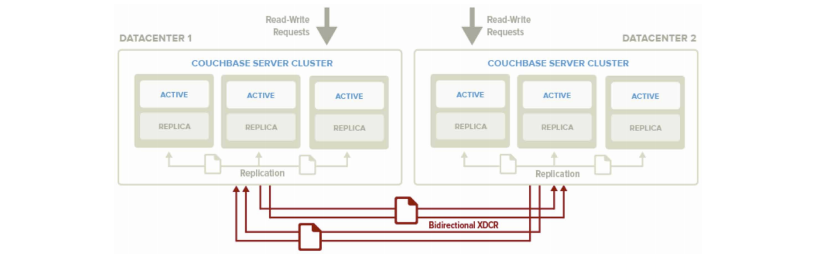
You can also see that XDCR and intra-cluster replication occurs simultaneously. Intra-cluster replication is taking place within the clusters at both Datacenter 1 and Datacenter 2, while at the same time XDCR is replicating documents across datacenters. Both datacenters are serving read and write requests from the application.
XDCR use cases
Disaster Recovery. Disaster can strike your datacenter at any time – often with little or no warning. With active-active cross datacenter replication in Couchbase Server, applications can read and write to any geo-location ensuring availability of data 24x365 even if an entire datacenter goes down.
Bringing Data Closer to Users. Interactive web applications demand low latency response times to deliver an awesome application experience. The best way to reduce latency is to bring relevant data closer to the user. For example, in online advertising, sub-millisecond latency is needed to make optimized decisions about real-time ad placements. XDCR can be used to bring post-processed user profile data closer to the user for low latency data access.
Data Replication for Development and Test Needs. Developers and testers often need to simulate production-like environments for troubleshooting or to produce a more reliable test. By using cross datacenter replication, you can create test clusters that host subset of your production data so that you can test code changes without interrupting production processing or risking data loss.
XDCR basic topologies
XDCR can be configured to support a variety of different topologies; the most common are unidirectional and bidirectional.
Unidirectional Replication is one-way replication, where active data gets replicated from the source cluster to the destination cluster. You may use unidirectional replication when you want to create an active offsite backup, replicating data from one cluster to a backup cluster.
Bidirectional Replication allows two clusters to replicate data with each other. Setting up bidirectional replication in Couchbase Server involves setting up two unidirectional replication links from one cluster to the other. This is useful when you want to load balance your workload across two clusters where each cluster bidirectionally replicates data to the other cluster.
In both topologies, data changes on the source cluster are replicated to the destination cluster only after they are persisted to disk. You can also have more than two datacenters and replicate data between all of them.
XDCR can be setup on a per bucket basis. A bucket is a logical container for documents in Couchbase Server. Depending on your application requirements, you might want to replicate only a subset of the data in Couchbase Server between two clusters. With XDCR you can selectively pick which buckets to replicate between two clusters in a unidirectional or bidirectional fashion. As shown in Figure 3, there is no XDCR between Bucket A (Cluster 1) and Bucket A (Cluster 2). Unidirectional XDCR is setup between Bucket B (Cluster 1) and Bucket B (Cluster 2). There is bidirectional XDCR between Bucket C (Cluster 1) and Bucket C (Cluster 2):
Cross datacenter replication in Couchbase Server involves replicating active data to multiple, geographically diverse datacenters either for disaster recovery or to bring data closer to its users for faster data access, as shown in below:

As shown above, after the document is stored in Couchbase Server and before XDCR replicates a document to other datacenters, a couple of things happen within each Couchbase Server node.
Each server in a Couchbase cluster has a managed cache. When an application stores a document in Couchbase Server it is written into the managed cache.
The document is added into the intra-cluster replication queue to be replicated to other servers within the cluster.
The document is added into the disk write queue to be asynchronously persisted to disk. The document is persisted to disk after the disk-write queue is flushed.
-
After the documents are persisted to disk, XDCR pushes the replica documents to other clusters. On the destination cluster, replica documents received will be stored in cache. This means that replica data on the destination cluster can undergo low latency read/write operations:
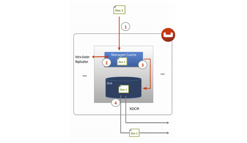
XDCR architecture
There are a number of key elements in Couchbase Server’s XDCR architecture including:
Continuous Replication. XDCR in Couchbase Server provides continuous replication across geographically distributed datacenters. Data mutations are replicated to the destination cluster after they are written to disk. There are multiple data streams (32 by default) that are shuffled across all shards (called vBuckets in Couchbase Server) on the source cluster to move data in parallel to the destination cluster. The vBucket list is shuffled so that replication is evenly load balanced across all the servers in the cluster. The clusters scale horizontally, more the servers, more the replication streams, faster the replication rate. For information on changing the number of data streams for replication, see Changing XDCR settings
Cluster Aware. XDCR is cluster topology aware. The source and destination clusters could have different number of servers. If a server in the source or destination cluster goes down, XDCR is able to get the updated cluster topology information and continue replicating data to available servers in the destination cluster.
Push based connection resilient replication. XDCR in Couchbase Server is push-based replication. The source cluster regularly checkpoints the replication queue per vBucket and keeps track of what data the destination cluster last received. If the replication process is interrupted for example due to a server crash or intermittent network connection failures, it is not required to restart replication from the beginning. Instead, once the replication link is restored, replication can continue from the last checkpoint seen by the destination cluster.
Efficient. For the sake of efficiency, Couchbase Server is able to de-duplicate information that is waiting to be stored on disk. For instance, if there are three changes to the same document in Couchbase Server, and these three changes are waiting in queue to be persisted, only the last version of the document is stored on disk and later gets pushed into the XDCR queue to be replicated.
Active-Active Conflict Resolution. Within a cluster, Couchbase Server provides strong consistency at the document level. On the other hand, XDCR also provides eventual consistency across clusters. Built-in conflict resolution will pick the same “winner” on both the clusters if the same document was mutated on both the clusters. If a conflict occurs, the document with the most updates will be considered the “winner.” If the same document is updated the same number of times on the source and destination, additional metadata such as numerical sequence, CAS value, document flags and expiration TTL value are used to pick the “winner.” XDCR applies the same rule across clusters to make sure document consistency is maintained:

As shown in above, bidirectional replication is set up between Datacenter 1 and Datacenter 2 and both the clusters start off with the same JSON document (Doc 1). In addition, two additional updates to Doc 1 happen on Datacenter 2. In the case of a conflict, Doc 1 on Datacenter 2 is chosen as the winner because it has seen more updates.
XDCR advanced topologies
By combining unidirectional and bidirectional topologies, you have the flexibility to create several complex topologies such as the chain and propagation topology as shown below:
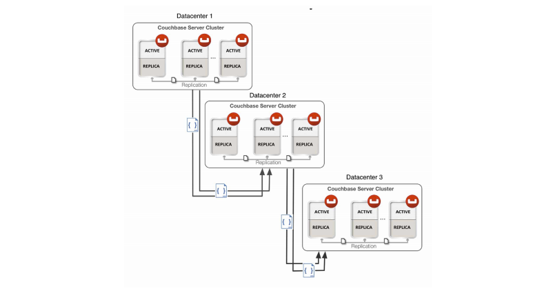
In the image below there is one bidirectional replication link between Datacenter 1 and Datacenter 2 and two unidirectional replication links between Datacenter 2 and Datacenters 3 and 4. Propagation replication can be useful in a scenario when you want to setup a replication scheme between two regional offices and several other local offices. Data between the regional offices is replicated bidirectionally between Datacenter 1 and Datacenter 2. Data changes in the local offices (Datacenters 3 and 4) are pushed to the regional office using unidirectional replication:
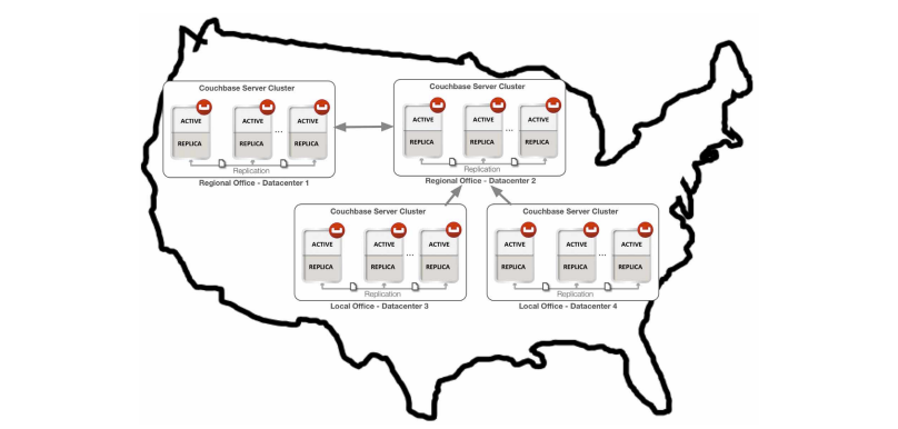
A description of the functionality, implementation and limitations of XDCR are provided in Behavior and Limitations.
To create and configure replication, see Configuring Replication.
XDCR behavior and limitations
This section discusses XDCR behavior and associated with various topics such as replication via memcached protocol, network or system outages, document handling and flush requests.
XDCR replication via memcached protocol
XDCR can replicate data through the memcached protocol at a destination cluster. This new mode utilizes highly efficient memcached protocol on the destination cluster for replicating changes. The new mode of XDCR increases XDCR throughput, reducing the CPU usage at destination cluster and also improves XDCR scalability.
In earlier versions of Couchbase Server only the REST protocol could be used for replication. On a source cluster a work process batched multiple mutations and sent the batch to a destination cluster using a REST interface. The REST interface at the destination node unpacked the batch of mutations and sent each mutation via a single memcached command. The destination cluster then stored mutations in RAM. This process is known as CAPI mode XDCR as it relies on the REST API known as CAPI.
This second mode available for XDCR is known as XMEM mode XDCR which bypasses the REST interface and replicates mutations via the memcached protocol at the destination cluster:
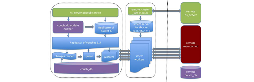
In this mode, every replication process at a source cluster delivers mutations directly via the memcached protocol on the remote cluster. This additional mode does not impact current XDCR architecture, rather it is implemented completely within the data communication layer used in XDCR. Any external XDCR interface remains the same. The benefit of using this mode is performance by increasing XDCR throughput, improving XDCR scalability, and reducing CPU usage at destination clusters during replication.
XDCR can be configured to operate via the new XMEM mode, which is the default or with CAPI mode. To change the replication mode, change the setting for
xdcr_replication_modevia the Web Console or REST API. For more information, see Changing Internal XDCRSettings.XDCR and network or system outages
XDCR is resilient to intermittent network failures. In the event that the destination cluster is unavailable due to a network interruption, XDCR pauses replication and then retries the connection to the cluster every 30 seconds. Once XDCR can successfully reconnect with a destination cluster, it resumes replication. In the event of a more prolonged network failure where the destination cluster is unavailable for more than 30 seconds, a source cluster continues polling the destination cluster which may result in numerous errors over time.
XDCR document handling
XDCR does not replicate views and view indexes. To replicate views and view indexes, manually exchange view definitions between clusters and re-generate the index on the destination cluster.
Non UTF-8 encodable document IDs on the source cluster are automatically filtered out and logged. The IDs are not transferred to the remote cluster. If there are any non UTF-8 keys, the warning output,
xdcr_error.*displays in the log files along with a list of all non-UTF-8 keys found by XDCR.XDCR flush requests
Flush requests to delete the entire contents of bucket are not replicated to the remote cluster. Performing a flush operation will only delete data on the local cluster. Flush is disabled if there is an active outbound replica stream configured.
Important
When replicating to or from a bucket, do not flush that bucket on the source or destination cluster. Flushing causes the vBucket state becomes temporarily unaccessible and results in a "not_found” error. The error suspends replication.
XDCR stream management
Under the following circumstances, a period of time should pass (depending on the CPU load) before creating new XDCR streams:
After creating a bucket After deleting an old XDCR stream
If a new XDCR stream is created immediately after a bucket has been created, a “db_not_found” error may occur. When a bucket is created, a period of time passes before the buckets are available. If XDCR tries to replicate to or from the vBucket too soon, a “db_not_found” error occurs. The same situation applies when other clients are “talking” to a bucket.
If a new XDCR stream is created immediately after an old XDCR stream is deleted, an Erlang eaddrinuse error occurs. This is related to the Erlang implementation of the TCP/IP protocol. After an Erlang process releases a socket, the socket stays in TIME_WAIT for a while before a new Erlang process can reuse it. If the new XDCR stream is created too quickly, vBucket replicators may encounter the eaddrinuse error and XDCR may not be able to fully start.
Note
The TIME_WAIT interval may be tunable from the operating system. If so, try lowering the interval time.
XDCR data encryption
The cross data center (XDCR) data security feature provides secure cross data center replication using Secure Socket Layer (SSL) data encryption. The data replicated between clusters can be encrypted in both uni-directional and bi-directional topologies.
By default, XDCR traffic to a destination cluster is sent in clear text that is unencrypted. In this case, when XDCR traffic occurs across multiple clusters over public networks, it is recommended that a VPN gateway be configured between the two data centers to encrypt the data between each route.
With the XDCR data encryption feature, the XDCR traffic from the source cluster is secured by enabling the XDCR encryption option, providing the destination cluster’s certificate, and then replicating.
Note
The certificate is an internal self-signed certificate used by SSL to initiate secure sessions. XDCR data encryption is supported only with Couchbase self-signed certificates. It does not support importing your own certificate files nor does it support signed certificates from a Certificate Authority (CA).
Data encryption is established between the source and destination clusters. Since data encryption is established at the cluster level, all buckets that are selected for replicated on the destination cluster are data encrypted. For buckets that need to be replicated without data encryption, establish a second XDCR destination cluster without XDCR data encryption enabled.
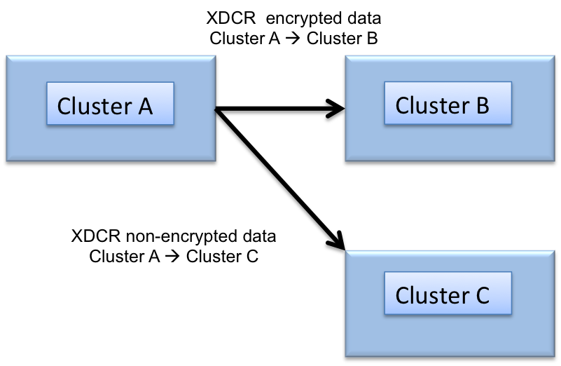
Important
Both data encrypted and non-encrypted replication can not occur between the same XDCR source and destination cluster. For example, if Cluster A (source) has data encryption enabled to Cluster B (destination), then Cluster A (source) cannot also have non-encryption (data encryption is *not* enabled) to Cluster B (destination).
For encrypted XDCR, the supported SSL/TLS-versions are SSL-3.0 and TLS-1.0. By default, XDCR uses the rc4-128 cipher suite, however, aes128 is used if rc4-128 isn’t available. XDCR can be forced to only use rc4-128 by setting the COUCHBASE_WANT_ARCFOUR environmental variable. OpenSSL is not used for the TLS/SSL handshake logic. Instead, the TLS/SSL logic is implemented in Erlang (see Heartbeat Bug and Couchbase Server blog. If specific ciphers/protocol/certificates are required, an alternative option is to connect to the clusters over an encrypted VPN connection.
For more information about enabling XDCR data encryption, see Managing XDCR data encryption.
Views and indexes
Views within Couchbase Server process the information stored in your Couchbase Server database, allowing you to index and query your data. A view creates an index on the stored information according to the format and structure defined within the view. The view consists of specific fields and information extracted from the objects stored in Couchbase. Views create indexes on your information allowing you to search and select information stored within Couchbase Server.
Note
Views are eventually consistent compared to the underlying stored documents. Documents are included in views when the document data is persisted to disk, and documents with expiry times are removed from indexes only when the expiration pager operates to remove the document from the database. For more information, read View Operation.
Views can be used within Couchbase Server for a number of reasons, including:
Indexing and querying data from your stored objects
Producing lists of data on specific object types
Producing tables and lists of information based on your stored data
Extracting or filtering information from the database
Calculating, summarizing or reducing the information on a collection of stored data
You can create multiple views and therefore multiple indexes and routes into the information stored in your database. By exposing specific fields from the stored information, views enable you to create and query the information stored within your Couchbase Server, perform queries and selection on the information, and paginate through the view output. The View Builder provides an interface for creating your views within the Couchbase Server Web Console. Views can be accessed using a suitable client library to retrieve matching records from the Couchbase Server database.
For background information on the creation of views and how they relate to the contents of your Couchbase Server database, see View Basics.
For more information on how views work with stored information, see Views and Stored Data.
For information on the rules and implementation of views, see View Operation.
Two types of views, development and production, are used to help optimize performance and view development. See Development and Production Views.
Writing views, including the language and options available are covered in Development and Production Views.
For a detailed background and technical information on troubleshooting views, see Troubleshooting Views (Technical Background).
The Couchbase Server Web Console includes an editor for writing and developing new views. See Using the Views Editor. You can also use a REST API to create, update and delete design documents. See the REST API, Design Documents.
View basics
The purpose of a view is take the un-structured, or semi-structured, data stored within your Couchbase Server database, extract the fields and information that you want, and to produce an index of the selected information. Storing information in Couchbase Server using JSON makes the process of selecting individual fields for output easier. The resulting generated structure is a view on the stored data. The view that is created during this process allows you to iterate, select and query the information in your database from the raw data objects that have been stored.
A brief overview of this process is shown in the figure below.
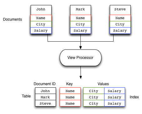
In the above example, the view takes the Name, City and Salary fields from the stored documents and then creates a array of this information for each document in the view. A view is created by iterating over every single document within the Couchbase bucket and outputting the specified information. The resulting index is stored for future use and updated with new data stored when the view is accessed. The process is incremental and therefore has a low ongoing impact on performance. Creating a new view on an existing large dataset may take a long time to build, but updates to the data will be quick.
The view definition specifies the format and content of the information generated for each document in the database. Because the process relies on the fields of stored JSON, if the document is not JSON, or the requested field in the view does not exist, the information is ignored. This enables the view to be created, even if some documents have minor errors or lack the relevant fields altogether.
One of the benefits of a document database is the ability to change the format of documents stored in the database at any time, without requiring a wholesale change to applications or a costly schema update before doing so.
View operation
All views within Couchbase operate as follows:
Views are updated when the document data is persisted to disk. There is a delay between creating or updating the document, and the document being updated within the view.
Documents that are stored with an expiry are not automatically removed until the background expiry process removes them from the database. This means that expired documents may still exist within the index.
Views are scoped within a design document, with each design document part of a single bucket. A view can only access the information within the corresponding bucket.
View names must be specified using one or more UTF-8 characters. You cannot have a blank view name. View names cannot have leading or trailing whitespace characters (space, tab, newline, or carriage-return).
Document IDs that are not UTF-8 encodable are automatically filtered and not included in any view. The filtered documents are logged so that they can be identified.
If you have a long view request, use POST instead of GET.
Views can only access documents defined within their corresponding bucket. You cannot access or aggregate data from multiple buckets within a given view.
-
Views are created as part of a design document, and each design document exists within the corresponding named bucket.
Each design document can have 0-n views.
Each bucket can contain 0-n design documents.
All the views within a single design document are updated when the update to a single view is triggered. For example, a design document with three views will update all three views simultaneously when just one of these views is updated.
-
Updates can be triggered in two ways:
At the point of access or query by using the
staleparameter (see Index Updates and the stale Parameter ).-
Automatically by Couchbase Server based on the number of updated documents, or the period since the last update.
Automatic updates can be controlled either globally, or individually on each design document. See Automated Index Updates.
-
Views are updated incrementally. The first time the view is accessed, all the documents within the bucket are processed through the map/reduce functions. Each new access to the view only processes the documents that have been added, updated, or deleted, since the last time the view index was updated.
In practice this means that views are entirely incremental in nature. Updates to views are typically quick as they only update changed documents. You should try to ensure that views are updated, using either the built-in automatic update system, through client-side triggering, or explicit updates within your application framework.
Because of the incremental nature of the view update process, information is only ever appended to the index stored on disk. This helps ensure that the index is updated efficiently. Compaction (including auto-compaction) will optimize the index size on disk and optimize the index structure. An optimized index is more efficient to update and query. See Database and View Compaction.
The entire view is recreated if the view definition has changed. Because this would have a detrimental effect on live data, only development views can be modified.
Note
Views are organized by design document, and indexes are created according to the design document. Changing a single view in a design document with multiple views invalidates all the views (and stored indexes) within the design document, and all the corresponding views defined in that design document will need to be rebuilt. This will increase the I/O across the cluster while the index is rebuilt, in addition to the I/O required for any active production views.
You can choose to update the result set from a view before you query it or after you query. Or you can choose to retrieve the existing result set from a view when you query the view. In this case the results are possibly out of date, or stale. For more information, see Index Updates and the stale Parameter.
The views engine creates an index is for each design document; this index contains the results for all the views within that design document.
-
The index information stored on disk consists of the combination of both the key and value information defined within your view. The key and value data is stored in the index so that the information can be returned as quickly as possible, and so that views that include a reduce function can return the reduced information by extracting that data from the index.
Because the value and key information from the defined map function are stored in the index, the overall size of the index can be larger than the stored data if the emitted key/value information is larger than the original source document data.
How expiration impacts views
Be aware that Couchbase Server does lazy expiration, that is, expired items are flagged as deleted rather than being immediately erased. Couchbase Server has a maintenance process, called expiry pager that will periodically look through all information and erase expired items. This maintenance process will run every 60 minutes, but it can be configured to run at a different interval. Couchbase Server will immediately remove an item flagged for deletion the next time the item requested; the server will respond that the item does not exist to the requesting process.
The result set from a view will contain any items stored on disk that meet the requirements of your views function. Therefore information that has not yet been removed from disk may appear as part of a result set when you query a view.
Using Couchbase views, you can also perform reduce functions on data, which perform calculations or other aggregations of data. For instance if you want to count the instances of a type of object, you would use a reduce function. Once again, if an item is on disk, it will be included in any calculation performed by your reduce functions. Based on this behavior due to disk persistence, here are guidelines on handling expiration with views:
-
Detecting Expired Documents in Result Sets : If you are using views for indexing items from Couchbase Server, items that have not yet been removed as part of the expiry pager maintenance process will be part of a result set returned by querying the view. To exclude these items from a result set you should use query parameter
include_docsset totrue. This parameter typically includes all JSON documents associated with the keys in a result set. For example, if you use the parameterinclude_docs=trueCouchbase Server will return a result set with an additional"doc"object which contains the JSON or binary data for that key:{"total_rows":2,"rows":[ {"id":"test","key":"test","value":null,"doc":{"meta":{"id":"test","rev":"4-0000003f04e86b040000000000000000","expiration":0,"flags":0},"json":{"testkey":"testvalue"}}}, {"id":"test2","key":"test2","value":null,"doc":{"meta":{"id":"test2","rev":"3-0000004134bd596f50bce37d00000000","expiration":1354556285,"flags":0},"json":{"testkey":"testvalue"}}} ] }For expired documents if you set
include_docs=true, Couchbase Server will return a result set indicating the document does not exist anymore. Specifically, the key that had expired but had not yet been removed by the cleanup process will appear in the result set as a row where"doc":null:{"total_rows":2,"rows":[ {"id":"test","key":"test","value":null,"doc":{"meta":{"id":"test","rev":"4-0000003f04e86b040000000000000000","expiration":0,"flags":0},"json":{"testkey":"testvalue"}}}, {"id":"test2","key":"test2","value":null,"doc":null} ] } -
Reduces and Expired Documents : In some cases, you may want to perform a reduce function to perform aggregations and calculations on data in Couchbase Server. In this case, Couchbase Server takes pre-calculated values which are stored for an index and derives a final result. This also means that any expired items still on disk will be part of the reduction. This may not be an issue for your final result if the ratio of expired items is proportionately low compared to other items. For instance, if you have 10 expired scores still on disk for an average performed over 1 million players, there may be only a minimal level of difference in the final result. However, if you have 10 expired scores on disk for an average performed over 20 players, you would get very different result than the average you would expect.
In this case, you may want to run the expiry pager process more frequently to ensure that items that have expired are not included in calculations used in the reduce function. We recommend an interval of 10 minutes for the expiry pager on each node of a cluster. Do note that this interval will have some slight impact on node performance as it will be performing cleanup more frequently on the node.
For more information about setting intervals for the maintenance process, refer to the Couchbase command line tool and review the examples on
exp_pager_stime.How views function in a cluster
Distributing data. If you familiar working with Couchbase Server you know that the server distributes data across different nodes in a cluster. This means that if you have four nodes in a cluster, on average each node will contain about 25% of active data. If you use views with Couchbase Server, the indexing process runs on all four nodes and the four nodes will contain roughly 25% of the results from indexing on disk. We refer to this index as a partial index, since it is an index based on a subset of data within a cluster. We show this in this partial index in the illustration below.
Replicating data and Indexes. Couchbase Server also provides data replication; this means that the server will replicate data from one node onto another node. In case the first node fails the second node can still handle requests for the data. To handle possible node failure, you can specify that Couchbase Server also replicate a partial index for replicated data. By default each node in a cluster will have a copy of each design document and view functions. If you make any changes to a views function, Couchbase Server will replicate this change to all nodes in the cluster. The sever will generate indexes from views within a single design document and store the indexes in a single file on each node in the cluster:
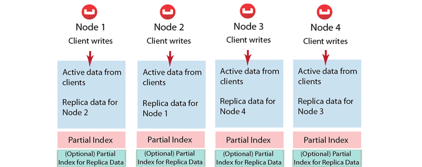
Couchbase Server can optionally create replica indexes on nodes that are contain replicated data; this is to prepare your cluster for a failover scenario. The server does not replicate index information from another node, instead each node creates an index for the replicated data it stores. The server recreates indexes using the replicated data on a node for each defined design document and view. By providing replica indexes the server enables you to still perform queries even in the event of node failure. You can specify whether Couchbase Server creates replica indexes or not when you create a data bucket. For more information, see Creating and Editing Data Buckets
Query Time within a Cluster
When you query a view and thereby trigger the indexing process, you send that request to a single node in the cluster. This node then distributes the request to all other nodes in the cluster. Depending on the parameter you send in your query, each node will either send the most current partial index at that node, will update the partial index and send it, or send the partial index and update it on disk. Couchbase Server will collect and collate these partial indexes and sent this aggregate result to a client.
To handle errors when you perform a query, you can configure how the cluster behaves when errors occur. See Error Control.
Queries During Rebalance or Failover
You can query an index during cluster rebalance and node failover operations. If you perform queries during rebalance or node failure, Couchbase Server will ensure that you receive the query results that you would expect from a node as if there were no rebalance or node failure.
During node rebalance, you will get the same results you would get as if the data were active data on a node and as if data were not being moved from one node to another. In other words, this feature ensures you get query results from a node during rebalance that are consistent with the query results you would have received from the node before rebalance started. This functionality operates by default in Couchbase Server, however you can optionally choose to disable it. Be aware that while this functionality, when enabled, will cause cluster rebalance to take more time; however we do not recommend you disable this functionality in production without thorough testing otherwise you may observe inconsistent query results.
View performance
View performance includes the time taken to update the view, the time required for the view update to be accessed, and the time for the updated information to be returned, depend on different factors. Your file system cache, frequency of updates, and the time between updating document data and accessing (or updating) a view will all impact performance.
Some key notes and points are provided below:
Index queries are always accessed from disk; indexes are not kept in RAM by Couchbase Server. However, frequently used indexes are likely to be stored in the filesystem cache used for caching information on disk. Increasing your filesystem cache, and reducing the RAM allocated to Couchbase Server from the total RAM available will increase the RAM available for the OS.
-
The filesystem cache will play a role in the update of the index information process. Recently updated documents are likely to be stored in the filesystem cache. Requesting a view update immediately after an update operation will likely use information from the filesystem cache. The eventual persistence nature implies a small delay between updating a document, it being persisted, and then being updated within the index.
Keeping some RAM reserved for your operating system to allocate filesystem cache, or increasing the RAM allocated to filesystem cache, will help keep space available for index file caching.
View indexes are stored, accessed, and updated, entirely independently of the document updating system. This means that index updates and retrieval is not dependent on having documents in memory to build the index information. Separate systems also mean that the performance when retrieving and accessing the cluster is not dependent on the document store.
Index updates and the stale parameter
Indexes are created by Couchbase Server based on the view definition, but updating of these indexes can be controlled at the point of data querying, rather than each time data is inserted. Whether the index is updated when queried can be controlled through the
staleparameter.Note
Irrespective of the
staleparameter, documents can only be indexed by the system once the document has been persisted to disk. If the document has not been persisted to disk, use of thestalewill not force this process. You can use theobserveoperation to monitor when documents are persisted to disk and/or updated in the index.Note
Views can also be updated automatically according to a document change, or interval count. See Automated Index Updates.
Three values for
staleare supported:-
stale=ok
The index is not updated. If an index exists for the given view, then the information in the current index is used as the basis for the query and the results are returned accordingly.
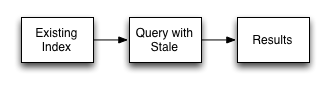
This setting results in the fastest response times to a given query, since the existing index will be used without being updated. However, this risks returning incomplete information if changes have been made to the database and these documents would otherwise be included in the given view.
-
stale=false
The index is updated before the query is executed. This ensures that any documents updated (and persisted to disk) are included in the view. The client will wait until the index has been updated before the query has executed, and therefore the response will be delayed until the updated index is available.
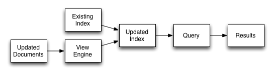
-
stale=update_after
This is the default setting if no
staleparameter is specified. The existing index is used as the basis of the query, but the index is marked for updating once the results have been returned to the client.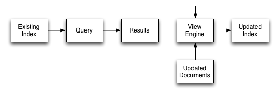
Warning
The indexing engine is an asynchronous process; this means querying an index may produce results you may not expect. For example, if you update a document, and then immediately run a query on that document you may not get the new information in the emitted view data. This is because the document updates have not yet been committed to disk, which is the point when the updates are indexed.
This also means that deleted documents may still appear in the index even after deletion because the deleted document has not yet been removed from the index.
For both scenarios, you should use an
observecommand from a client with thempersisttoargument to verify the persistent state for the document, then force an update of the view usingstale=false. This will ensure that the document is correctly updated in the view index.When you have multiple clients accessing an index, the index update process and results returned to clients depend on the parameters passed by each client and the sequence that the clients interact with the server.
-
Situation 1
Client 1 queries view with
stale=falseClient 1 waits until server updates the index
Client 2 queries view with
stale=falsewhile re-indexing from Client 1 still in progressClient 2 will wait until existing index process triggered by Client 1 completes. Client 2 gets updated index.
-
Situation 2
Client 1 queries view with
stale=falseClient 1 waits until server updates the index
Client 2 queries view with
stale=okwhile re-indexing from Client 1 in progressClient 2 will get the existing index
-
Situation 3
Client 1 queries view with
stale=falseClient 1 waits until server updates the index
Client 2 queries view with
stale=update_afterIf re-indexing from Client 1 not done, Client 2 gets the existing index. If re-indexing from Client 1 done, Client 2 gets this updated index and triggers re-indexing.
Note
Index updates may be stacked if multiple clients request that the view is updated before the information is returned (
stale=false). This ensures that multiple clients updating and querying the index data get the updated document and version of the view each time. Forstale=update_afterqueries, no stacking is performed, since all updates occur after the query has been accessed.Sequential accesses
Client 1 queries view with stale=ok
Client 2 queries view with stale=false
View gets updated
Client 1 queries a second time view with stale=ok
Client 1 gets the updated view version
The above scenario can cause problems when paginating over a number of records as the record sequence may change between individual queries.
Automated index updates
In addition to a configurable update interval, you can also update all indexes automatically in the background. You configure automated update through two parameters, the update time interval in seconds and the number of document changes that occur before the views engine updates an index. These two parameters are
updateIntervalandupdateMinChanges:updateInterval: the time interval in milliseconds, default is 5000 milliseconds. At everyupdateIntervalthe views engine checks if the number of document mutations on disk is greater thanupdateMinChanges. If true, it triggers view update. The documents stored on disk potentially lag documents that are in-memory for tens of seconds.updateMinChanges: the number of document changes that occur before re-indexing occurs, default is 5000 changes.
The auto-update process only operates on full-set development and production indexes. Auto-update does not operate on partial set development indexes.
Note
Irrespective of the automated update process, documents can only be indexed by the system once the document has been persisted to disk. If the document has not been persisted to disk, the automated update process will not force the unwritten data to be written to disk. You can use the
observeoperation to monitor when documents have been persisted to disk and/or updated in the index.The updates are applied as follows:
-
Active indexes, Production views
For all active, production views, indexes are automatically updated according to the update interval
updateIntervaland the number of document changesupdateMinChanges.If
updateMinChangesis set to 0 (zero), then automatic updates are disabled for main indexes. -
Replica indexes
If replica indexes have been configured for a bucket, the index is automatically updated according to the document changes (
replicaUpdateMinChanges; default 5000) settings.If
replicaUpdateMinChangesis set to 0 (zero), then automatic updates are disabled for replica indexes.
The trigger level can be configured both globally and for individual design documents for all indexes using the REST API.
To obtain the current view update daemon settings, access a node within the cluster on the administration port using the URL
http://nodename:8091/settings/viewUpdateDaemon:GET http://Administrator:Password@nodename:8091/settings/viewUpdateDaemonThe request returns the JSON of the current update settings:
{
    "updateInterval":5000,
    "updateMinChanges":5000,
    "replicaUpdateMinChanges":5000
}
To update the settings, use
POSTwith a data payload that includes the updated values. For example, to update the time interval to 10 seconds, and document changes to 7000 each:POST http://nodename:8091/settings/viewUpdateDaemon updateInterval=10000&updateMinChanges=7000If successful, the return value is the JSON of the updated configuration.
To configure the updateMinChanges or replicaUpdateMinChanges values explicitly on individual design documents, you must specify the parameters within the
optionssection of the design document. For example:{ "_id": "_design/myddoc", "views": { "view1": { "map": "function(doc, meta) { if (doc.value) { emit(doc.value, meta.id);} }" } }, "options": { "updateMinChanges": 1000, "replicaUpdateMinChanges": 20000 } }You can set this information when creating and updating design documents through the design document REST API. For more information, see Storing design documents.
To perform this operation using the
curltool:> curl -X POST -v -d 'updateInterval=7000&updateMinChanges=7000' \ 'http://Administrator:Password@192.168.0.72:8091/settings/viewUpdateDaemon'Partial-set development views are not automatically rebuilt, and during a rebalance operation, development views are not updated, even when when consistent views are enabled, as this relies on the automated update mechanism. Updating development views in this way would waste system resources.
Views and stored data
The view system relies on the information stored within your cluster being formatted as a JSON document. The formatting of the data in this form allows the individual fields of the data to be identified and used at the components of the index.
Information is stored into your Couchbase database the data stored is parsed, if the information can be identified as valid JSON then the information is tagged and identified in the database as valid JSON. If the information cannot be parsed as valid JSON then it is stored as a verbatim binary copy of the submitted data.
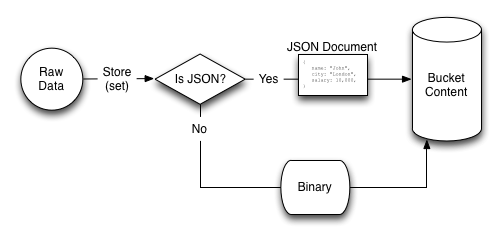
When retrieving the stored data, the format of the information depends on whether the data was tagged as valid JSON or not:
-
JSON
Information identified as JSON data may not be returned in a format identical to that stored. The information will be semantically identical, in that the same fields, data and structure as submitted will be returned. Metadata information about the document is presented in a separate structure available during view processing.
The white space, field ordering may differ from the submitted version of the JSON document.
For example, the JSON document below, stored using the key
mykey:{ "title" : "Fish Stew", "servings" : 4, "subtitle" : "Delicious with fresh bread" }May be returned within the view processor as:
{ "servings": 4, "subtitle": "Delicious with fresh bread", "title": "Fish Stew" } -
Non-JSON
Information not parsable as JSON will always be stored and returned as a binary copy of the information submitted to the database. If you store an image, for example, the data returned will be an identical binary copy of the stored image.
Non-JSON data is available as a base64 string during view processing. A non-JSON document can be identified by examining the
typefield of the metadata structure.
The significance of the returned structure can be seen when editing the view within the Web Console.
JSON basics
JSON is used because it is a lightweight, easily parsed, cross-platform data representation format. There are a multitude of libraries and tools designed to help developers work efficiently with data represented in JSON format, on every platform and every conceivable language and application framework, including, of course, most web browsers.
JSON supports the same basic types as supported by JavaScript, these are:
-
Number (either integer or floating-point).
JavaScript supports a maximum numerical value of 253. If you are working with numbers larger than this from within your client library environment (for example, 64-bit numbers), you must store the value as a string.
-
String — this should be enclosed by double-quotes and supports Unicode characters and backslash escaping. For example:
"A String" -
Boolean — a
trueorfalsevalue. You can use these strings directly. For example:{ "value": true} -
Array — a list of values enclosed in square brackets. For example:
["one", "two", "three"] -
Object — a set of key/value pairs (i.e. an associative array, or hash). The key must be a string, but the value can be any of the supported JSON values. For example:
{
    "servings" : 4,
    "subtitle" : "Easy to make in advance, and then cook when ready",
    "cooktime" : 60,
    "title" : "Chicken Coriander"
 }
If the submitted data cannot be parsed as a JSON, the information will be stored as a binary object, not a JSON document.
Warning
If the submitted data cannot be parsed as a JSON, the information will be stored as a binary object, not a JSON document.
Document metadata
During view processing, metadata about individual documents is exposed through a separate JSON object,
meta, that can be optionally defined as the second argument to themap(). This metadata can be used to further identify and qualify the document being processed.The
metastructure contains the following fields and associated information:-
idThe ID or key of the stored data object. This is the same as the key used when writing the object to the Couchbase database.
-
revAn internal revision ID used internally to track the current revision of the information. The information contained within this field is not consistent or trackable and should not be used in client applications.
-
typeThe type of the data that has been stored. A valid JSON document will have the type
json. Documents identified as binary data will have the typebase64. -
flagsThe numerical value of the flags set when the data was stored. The availability and value of the flags is dependent on the client library you are using to store your data. Internally the flags are stored as a 32-bit integer.
-
expirationThe expiration value for the stored object. The stored expiration time is always stored as an absolute Unix epoch time value.
Note
These additional fields are only exposed when processing the documents within the view server. These fields are not returned when you access the object through the Memcached/Couchbase protocol as part of the document.
Non-JSON data
All documents stored in Couchbase Server will return a JSON structure, however, only submitted information that could be parsed into a JSON document will be stored as a JSON document. If you store a value that cannot be parsed as a JSON document, the original binary data is stored. This can be identified during view processing by using the
metaobject supplied to themap()function.Note
Information that has been identified and stored as binary documents instead of JSON documents can still be indexed through the views system by creating an index on the key data. This can be particularly useful when the document key is significant. For example, if you store information using a prefix to the key to identify the record type, you can create document-type specific indexes.
For more information and examples, see Views on non-JSON Data.
Document storage and indexing sequence
The method of storage of information into the Couchbase Server affects how and when the indexing information is built, and when data written to the cluster is incorporated into the indexes. In addition, the indexing of data is also affected by the view system and the settings used when the view is accessed.
The basic storage and indexing sequence is:
A document is stored within the cluster. Initially the document is stored only in RAM.
The document is persisted to disk through the standard disk write queue mechanism.
Once the document has been persisted to disk, the document can be indexed by the view mechanism.
This sequence means that the view results are
eventually consistentwith what is stored in memory based on whether documents have been persisted to disk. It is possible to write a document to the cluster, and access the index, without the newly written document appearing in the generated view index.Conversely, documents that have been stored with an expiry may continue to be included within the view index until the document has been removed from the database by the expiry pager.
Note
Couchbase Server supports the Observe command, which enables the current state of a document and whether the document has been persisted to disk and/or whether it has been considered for inclusion in an index.
When accessing a view, the contents of the view are asynchronous to the stored documents. In addition, the creation and updating of the view is subject to the
staleparameter. This controls how and when the view is updated when the view content is queried. For more information, see Index Updates and the stale Parameter. Views can also be automatically updated on a schedule so that their data is not too out of sync with stored documents. For more information, see Automated Index Updates.Development and production views
Due to the nature of the Couchbase cluster and because of the size of the datasets that can be stored across a cluster, the impact of view development needs to be controlled. Creating a view implies the creation of the index which could slow down the performance of your server while the index is being generated. However, views also need to be built and developed using the actively stored information.
To support both the creation and testing of views, and the deployment of views in production, Couchbase Server supports two different view types,Developmentviews andProductionviews. The two view types work identically, but have different purposes and restrictions placed upon their operation.
-
Development views
Development views are designed to be used while you are still selecting and designing your view definitions. While a view is in development mode, views operate with the following attributes
By default the development view works on only a subset of the stored information. You can, however, force the generation of a development view information on the full dataset.
Development views use live data from the selected Couchbase bucket, enabling you to develop and refine your view in real-time on your production data.
Development views are not automatically rebuilt, and during a rebalance operation, development views are not updated, even when when consistent views are enabled, as this relies on the automated update mechanism. Updating development views in this way would waste system resources.
Development views are fully editable and modifiable during their lifetime. You can change and update the view definition for a development view at any time.
During development of the view, you can view and edit stored document to help develop the view definition.
Development views are accessed from client libraries through a different URL than production views, making it easy to determine the view type and information during development of your application.
-
Within the Web Console, the execution of a view by default occurs only over a subset of the full set of documents stored in the bucket. You can elect to run the View over the full set using the Web Console.
Warning
Because of the selection process, the reduced set of documents may not be fully representative of all the documents in the bucket. You should always check the view execution over the full set.
-
Production views
Production views are optimized for production use. A production view has the following attributes:
Production views always operate on the full dataset for their respective bucket.
Production views can either be created from the Web Console or through REST API. From the Web Console, you first create development views and then publish them as production views. Through REST API, you directly create the production views (and skip the initial development views).
-
Production views cannot be modified through the UI. You can only access the information exposed through a production view. To make changes to a production view, it must be copied to a development view, edited, and re-published.
Views can be updated by the REST API, but updating a production design document immediately invalidates all of the views defined within it.
Production views are accessed through a different URL to development views.
The support for the two different view types means that there is a typical work flow for view development, as shown in the figure below:
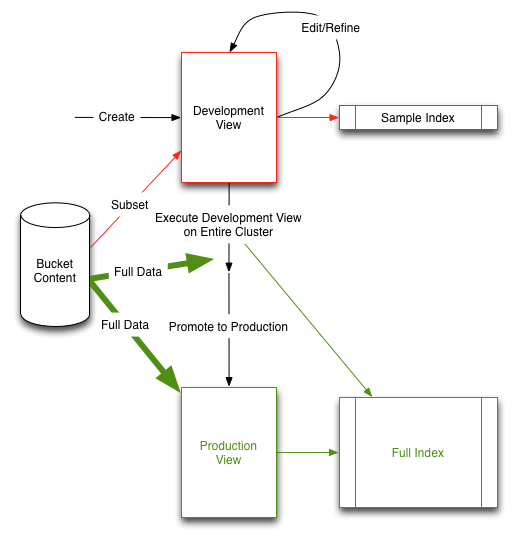
The above diagram features the following steps:
Create a development view and view the sample view output.
-
Refine and update your view definition to suit your needs, repeating the process until your view is complete.
During this phase you can access your view from your client library and application to ensure it suits your needs.
Once the view definition is complete, apply your view to your entire Cluster dataset.
Push your development view into production. This moves the view from development into production, and renames the index (so that the index does not need to be rebuilt).
Start using your production view.
Individual views are created as part of a design document. Each design document can have multiple views, and each Couchbase bucket can have multiple design documents. You can therefore have both development and production views within the same bucket while you development different indexes on your data.
For information on publishing a view from development to production state, see Publishing Views.
Writing views
The fundamentals of a view are straightforward. A view creates a perspective on the data stored in your Couchbase buckets in a format that can be used to represent the data in a specific way, define and filter the information, and provide a basis for searching or querying the data in the database based on the content. During the view creation process, you define the output structure, field order, content and any summary or grouping information desired in the view.
Views achieve this by defining an output structure that translates the stored JSON object data into a JSON array or object across two components, the key and the value. This definition is performed through the specification of two separate functions written in JavaScript. The view definition is divided into two parts, a map function and a reduce function:
-
Map function
As the name suggests, the map function creates a mapping between the input data (the JSON objects stored in your database) and the data as you want it displayed in the results (output) of the view. Every document in the Couchbase bucket for the view is submitted to the
map()function in each view once, and it is the output from themap()function that is used as the result of the view.The
map()function is supplied two arguments by the views processor. The first argument is the JSON document data. The optional second argument is the associated metadata for the document, such as the expiration, flags, and revision information.The map function outputs zero or more ‘rows’ of information using an
emit()function. Each call to theemit()function is equivalent to a row of data in the view result. Theemit()function can be called multiple times within the single pass of themap()function. This functionality allows you to create views that may expose information stored in a compound format within a single stored JSON record, for example generating a row for each item in an array.You can see this in the figure below, where the name, salary and city fields of the stored JSON documents are translated into a table (an array of fields) in the generated view content.
-
Reduce function
The reduce function is used to summarize the content generated during the map phase. Reduce functions are optional in a view and do not have to be defined. When they exist, each row of output (from each
emit()call in the correspondingmap()function) is processed by the correspondingreduce()function.If a reduce function is specified in the view definition it is automatically used. You can access a view without enabling the reduce function by disabling reduction (
reduce=false) when the view is accessed.Typical uses for a reduce function are to produce a summarized count of the input data, or to provide sum or other calculations on the input data. For example, if the input data included employee and salary data, the reduce function could be used to produce a count of the people in a specific location, or the total of all the salaries for people in those locations.
The combination of the map and the reduce function produce the corresponding view. The two functions work together, with the map producing the initial material based on the content of each JSON document, and the reduce function summarizing the information generated during the map phase. The reduction process is selectable at the point of accessing the view, you can choose whether to the reduce the content or not, and, by using an array as the key, you can specifying the grouping of the reduce information.
Each row in the output of a view consists of the view key and the view value. When accessing a view using only the map function, the contents of the view key and value are those explicitly stated in the definition. In this mode the view will also always contain an
idfield which contains the document ID of the source record (i.e. the string used as the ID when storing the original data record).When accessing a view employing both the map and reduce functions the key and value are derived from the output of the reduce function based on the input key and group level specified. A document ID is not automatically included because the document ID cannot be determined from reduced data where multiple records may have been merged into one. Examples of the different explicit and implicit values in views will be shown as the details of the two functions are discussed.
You can see an example of the view creation process in the figure below.
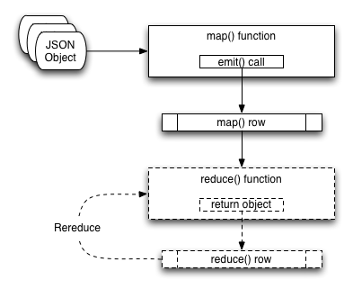
Because of the separation of the two elements, you can consider the two functions individually.
For information on how to write map functions, and how the output of the map function affects and supports searching, see Map functions. For details on writing the reduce function, see Reduce functions.
Note
View names must be specified using one or more UTF-8 characters. You cannot have a blank view name. View names cannot have leading or trailing whitespace characters (space, tab, newline, or carriage-return).
To create views, you can use either the Admin Console View editor (see Using the Views Editor ), use the REST API for design documents (see the REST API, Design Documents ), or use one of the client libraries that support view management.
For more information and examples on how to query and obtain information from a map, see Querying Views.
Map functions
The map function is the most critical part of any view as it provides the logical mapping between the input fields of the individual objects stored within Couchbase to the information output when the view is accessed.
Through this mapping process, the map function and the view provide:
The output format and structure of the view on the bucket.
Structure and information used to query and select individual documents using the view information.
Sorting of the view results.
Input information for summarizing and reducing the view content.
Applications access views through the REST API, or through a Couchbase client library. All client libraries provide a method for submitting a query into the view system and obtaining and processing the results.
The basic operation of the map function can be seen in the figure below.
In this example, a map function is taking the Name, City, and Salary fields from the JSON documents stored in the Couchbase bucket and mapping them to a table of these fields. The map function which produces this output might look like this:
function(doc, meta)
{
  emit(doc.name, [doc.city, doc.salary]);
}
When the view is generated the
map()function is supplied two arguments for each stored document,docandmeta:-
docThe stored document from the Couchbase bucket, either the JSON or binary content. Content type can be identified by accessing the
typefield of themetaargument object. -
metaThe metadata for the stored document, containing expiry time, document ID, revision and other information. For more information, see Document Metadata.
Every document in the Couchbase bucket is submitted to the
map()function in turn. After the view is created, only the documents created or changed since the last update need to be processed by the view. View indexes and updates are materialized when the view is accessed. Any documents added or changed since the last access of the view will be submitted to themap()function again so that the view is updated to reflect the current state of the data bucket.Within the
map()function itself you can perform any formatting, calculation or other detail. To generate the view information, you use calls to theemit()function. Each call to theemit()function outputs a single row or record in the generated view content.The
emit()function accepts two arguments, the key and the value for each record in the generated view:-
key
The emitted key is used by Couchbase Server both for sorting and querying the content in the database.
The key can be formatted in a variety of ways, including as a string or compound value (such as an array or JSON object). The content and structure of the key is important, because it is through the emitted key structure that information is selected within the view.
All views are output in a sorted order according to the content and structure of the key. Keys using a numeric value are sorted numerically, for strings, UTF-8 is used. Keys can also support compound values such as arrays and hashes. For more information on the sorting algorithm and sequence, see Ordering.
The key content is used for querying by using a combination of this sorting process and the specification of either an explicit key or key range within the query specification. For example, if a view outputs the
RECIPE TITLEfield as a key, you could obtain all the records matching ‘Lasagne’ by specifying that only the keys matching ‘Lasagne’ are returned.For more information on querying and extracting information using the key value, see Querying Views.
-
value
The value is the information that you want to output in each view row. The value can be anything, including both static data, fields from your JSON objects, and calculated values or strings based on the content of your JSON objects.
The content of the value is important when performing a reduction, since it is the value that is used during reduction, particularly with the built-in reduction functions. For example, when outputting sales data, you might put the
SALESMANinto the emitted key, and put the sales amounts into the value. The built-in_sumfunction will then total up the content of the corresponding value for each unique key.
The format of both key and value is up to you. You can format these as single values, strings, or compound values such as arrays or JSON. The structure of the key is important because you must specify keys in the same format as they were generated in the view specification.
The
emit()function can be called multiple times in a single map function, with each call outputting a single row in the generated view. This can be useful when you want to supporting querying information in the database based on a compound field. For a sample view definition and selection criteria, see Emitting Multiple Rows.Views and map generation are also very forgiving. If you elect to output fields in from the source JSON objects that do not exist, they will simply be replaced with a
nullvalue, rather than generating an error.For example, in the view below, some of the source records do contain all of the fields in the specified view. The result in the view result is just the
nullentry for that field in the value output.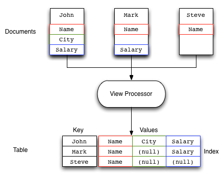
Note
You should check that the field or data source exists during the map processing before emitting the data.
To better understand how the map function works to output different types of information and retrieve it, see View and Query Pattern Samples.
Reduce functions
Often the information that you are searching or reporting on needs to be summarized or reduced. There are a number of different occasions when this can be useful. For example, if you want to obtain a count of all the items of a particular type, such as comments, recipes matching an ingredient, or blog entries against a keyword.
Note
When using a reduce function in your view, the value that you specify in the call to
emit()is replaced with the value generated by the reduce function. This is because the value specified byemit()is used as one of the input parameters to the reduce function. The reduce function is designed to reduce a group of values emitted by the correspondingmap()function.Alternatively, reduce can be used for performing sums, for example totalling all the invoice values for a single client, or totalling up the preparation and cooking times in a recipe. Any calculation that can be performed on a group of the emitted data.
In each of the above cases, the raw data is the information from one or more rows of information produced by a call to
emit(). The input data, each record generated by theemit()call, is reduced and grouped together to produce a new record in the output.The grouping is performed based on the value of the emitted key, with the rows of information generated during the map phase being reduced and collated according to the uniqueness of the emitted key.
When using a reduce function the reduction is applied as follows:
-
For each record of input, the corresponding reduce function is applied on the row, and the return value from the reduce function is the resulting row.
For example, using the built-in
_sumreduce function, thevaluein each case would be totaled based on the emitted key:{ "rows" : [ {"value" : 13000, "id" : "James", "key" : "James" }, {"value" : 20000, "id" : "James", "key" : "James" }, {"value" : 5000, "id" : "Adam", "key" : "Adam" }, {"value" : 8000, "id" : "Adam", "key" : "Adam" }, {"value" : 10000, "id" : "John", "key" : "John" }, {"value" : 34000, "id" : "John", "key" : "John" } ] }Using the unique key of the name, the data generated by the map above would be reduced, using the key as the collator, to the produce the following output:
{
     "rows" : [
        {"value" : 33000, "key" : "James" },
        {"value" : 13000, "key" : "Adam"  },
        {"value" : 44000, "key" : "John"  },
     ]
  }
In each case the values for the common keys (John, Adam, James), have been totalled, and the six input rows reduced to the 3 rows shown here.
Results are grouped on the key from the call to
emit()if grouping is selected during query time. As shown in the previous example, the reduction operates by the taking the key as the group value as using this as the basis of the reduction.If you use an array as the key, and have selected the output to be grouped during querying you can specify the level of the reduction function, which is analogous to the element of the array on which the data should be grouped. For more information, see Grouping in Queries.
The view definition is flexible. You can select whether the reduce function is applied when the view is accessed. This means that you can access both the reduced and unreduced (map-only) content of the same view. You do not need to create different views to access the two different types of data.
Whenever the reduce function is called, the generated view content contains the same key and value fields for each row, but the key is the selected group (or an array of the group elements according to the group level), and the value is the computed reduction value.
Couchbase includes the following built-in reduce functions:
You can also write your own custom reduction functions.
The reduce function also has a final additional benefit. The results of the computed reduction are stored in the index along with the rest of the view information. This means that when accessing a view with the reduce function enabled, the information comes directly from the index content. This results in a very low impact on the Couchbase Server to the query (the value is not computed at runtime), and results in very fast query times, even when accessing information based on a range-based query.
Note
The
reduce()function is designed to reduce and summarize the data emitted during themap()phase of the process. It should only be used to summarize the data, and not to transform the output information or concatenate the information into a single structure.When using a composite structure, the size limit on the composite structure within the
reduce()function is 64KB.Built-in _count
The
_countfunction provides a simple count of the input rows from themap()function, using the keys and group level to provide a count of the correlated items. The values generated during themap()stage are ignored.For example, using the input:
{
   "rows" : [
      {"value" : 13000, "id" : "James", "key" : ["James", "Paris"] },
      {"value" : 20000, "id" : "James", "key" : ["James", "Tokyo"] },
      {"value" : 5000,  "id" : "James", "key" : ["James", "Paris"] },
      {"value" : 7000,  "id" : "Adam",  "key" : ["Adam",  "London"] },
      {"value" : 19000, "id" : "Adam",  "key" : ["Adam",  "Paris"] },
      {"value" : 17000, "id" : "Adam",  "key" : ["Adam",  "Tokyo"] },
      {"value" : 22000, "id" : "John",  "key" : ["John",  "Paris"] },
      {"value" : 3000,  "id" : "John",  "key" : ["John",  "London"] },
      {"value" : 7000,  "id" : "John",  "key" : ["John",  "London"] },
    ]
}
Enabling the
reduce()function and using a group level of 1 would produce:{ "rows" : [ {"value" : 3, "key" : ["Adam" ] }, {"value" : 3, "key" : ["James"] }, {"value" : 3, "key" : ["John" ] } ] }The reduction has produce a new result set with the key as an array based on the first element of the array from the map output. The value is the count of the number of records collated by the first element.
Using a group level of 2 would generate the following:
{
   "rows" : [
      {"value" : 1, "key" : ["Adam", "London"] },
      {"value" : 1, "key" : ["Adam", "Paris" ] },
      {"value" : 1, "key" : ["Adam", "Tokyo" ] },
      {"value" : 2, "key" : ["James","Paris" ] },
      {"value" : 1, "key" : ["James","Tokyo" ] },
      {"value" : 2, "key" : ["John", "London"] },
      {"value" : 1, "key" : ["John", "Paris" ] }
   ]
}
Now the counts are for the keys matching both the first two elements of the map output.
Built-in _sum
The built-in
_sumfunction sums the values from themap()function call, this time summing up the information in the value for each row. The information can either be a single number or during a rereduce an array of numbers.Note
The input values must be a number, not a string-representation of a number. The entire map/reduce will fail if the reduce input is not in the correct format. You should use the
parseInt()orparseFloat()function calls within yourmap()function stage to ensure that the input data is a number.For example, using the same sales source data, accessing the group level 1 view would produce the total sales for each salesman:
{
   "rows" : [
      {"value" : 43000, "key" : [ "Adam"  ] },
      {"value" : 38000, "key" : [ "James" ] },
      {"value" : 32000, "key" : [ "John"  ] }
   ]
}
Using a group level of 2 you get the information summarized by salesman and city:
{
   "rows" : [
      {"value" : 7000,  "key" : [ "Adam",  "London" ] },
      {"value" : 19000, "key" : [ "Adam",  "Paris"  ] },
      {"value" : 17000, "key" : [ "Adam",  "Tokyo"  ] },
      {"value" : 18000, "key" : [ "James", "Paris"  ] },
      {"value" : 20000, "key" : [ "James", "Tokyo"  ] },
      {"value" : 10000, "key" : [ "John",  "London" ] },
      {"value" : 22000, "key" : [ "John",  "Paris"  ] }
   ]
}
Built-in _stats
The built-in
_statsreduce function produces statistical calculations for the input data. As with the_sumfunction, the corresponding value in the emit call should be a number. The generated statistics include the sum, count, minimum (min), maximum (max) and sum squared (sumsqr) of the input rows.Using the sales data, a slightly truncated output at group level one would be:
{
   "rows" : [
      {
         "value" : {
            "count" : 3,
            "min" : 7000,
            "sumsqr" : 699000000,
            "max" : 19000,
            "sum" : 43000
         },
         "key" : [
            "Adam"
         ]
      },
      {
         "value" : {
            "count" : 3,
            "min" : 5000,
            "sumsqr" : 594000000,
            "max" : 20000,
            "sum" : 38000
         },
         "key" : [
            "James"
         ]
      },
      {
         "value" : {
            "count" : 3,
            "min" : 3000,
            "sumsqr" : 542000000,
            "max" : 22000,
            "sum" : 32000
         },
         "key" : [
            "John"
         ]
      }
   ]
}
The same fields in the output value are provided for each of the reduced output rows.
Writing custom reduce functions
The
reduce()function has to work slightly differently to themap()function. In the primary form, areduce()function must convert the data supplied to it from the correspondingmap()function.The core structure of the reduce function execution is shown the figure below.
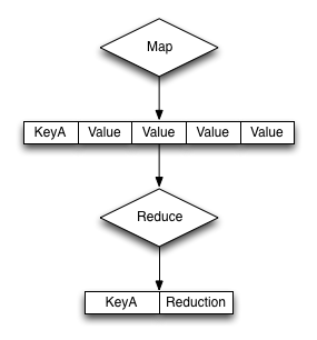
The base format of the
reduce()function is as follows:function(key, values, rereduce) { … return retval; }The reduce function is supplied three arguments:
-
keyThe
keyis the unique key derived from themap()function and thegroup_levelparameter. -
valuesThe
valuesargument is an array of all of the values that match a particular key. For example, if the same key is output three times,datawill be an array of three items containing, with each item containing the value output by theemit()function. -
rereduceThe
rereduceindicates whether the function is being called as part of a re-reduce, that is, the reduce function being called again to further reduce the input data.When
rereduceis false:The supplied
keyargument will be an array where the first argument is thekeyas emitted by the map function, and theidis the document ID that generated the key.The values is an array of values where each element of the array matches the corresponding element within the array of
keys.
When
rereduceis true:keywill be null.valueswill be an array of values as returned by a previousreduce()function.
The function returns the reduced version of the information. The format of the return value should match the format required for the specified key.
Re-writing the built-in reduce functions
Using this model as a template, it is possible to write the full implementation of the built-in functions
_sumand_countwhen working with the sales data and the standardmap()function below:function(doc, meta) { emit(meta.id, null); }The
_countfunction returns a count of all the records for a given key. Since argument for the reduce function contains an array of all the values for a given key, the length of the array needs to be returned in thereduce()function:function(key, values, rereduce) { if (rereduce) { var result = 0; for (var i = 0; i < values.length; i++) { result += values[i]; } return result; } else { return values.length; } }To explicitly write the equivalent of the built-in
_sumreduce function, the sum of supplied array of values needs to be returned:function(key, values, rereduce) { var sum = 0; for(i=0; i < values.length; i++) { sum = sum + values[i]; } return(sum); }In the above function, the array of data values is iterated over and added up, with the final value being returned.
Handling re-reduce
For
reduce()functions, they should be both transparent and standalone. For example, the_sumfunction did not rely on global variables or parsing of existing data, and didn’t need to call itself, hence it is also transparent.In order to handle incremental map/reduce functionality (i.e. updating an existing view), each function must also be able to handle and consume the functions own output. This is because in an incremental situation, the function must be handle both the new records, and previously computed reductions.
This can be explicitly written as follows:
f(keys, values) = f(keys, [ f(keys, values) ])This can been seen graphically in the illustration below, where previous reductions are included within the array of information are re-supplied to the reduce function as an element of the array of values supplied to the reduce function.
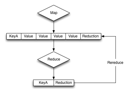
That is, the input of a reduce function can be not only the raw data from the map phase, but also the output of a previous reduce phase. This is called
rereduce, and can be identified by the third argument to thereduce(). When therereduceargument is true, both thekeyandvaluesarguments are arrays, with the corresponding element in each containing the relevant key and value. I.e.,key[1]is the key related to the value ofvalue[1].An example of this can be seen by considering an expanded version of the
sumfunction showing the supplied values for the first iteration of the view index building:function('James', [ 13000,20000,5000 ]) {...}When a document with the ‘James’ key is added to the database, and the view operation is called again to perform an incremental update, the equivalent call is:
function('James', [ 19000, function('James', [ 13000,20000,5000 ]) ]) { ... }In reality, the incremental call is supplied the previously computed value, and the newly emitted value from the new document:
function('James', [ 19000, 38000 ]) { ... }Fortunately, the simplicity of the structure for
summeans that the function both expects an array of numbers, and returns a number, so these can easily be recombined.If writing more complex reductions, where a compound key is output, the
reduce()function must be able to handle processing an argument of the previous reduction as the compound value in addition to the data generated by themap()phase. For example, to generate a compound output showing both the total and count of values, a suitablereduce()function could be written like this:function(key, values, rereduce) { var result = {total: 0, count: 0}; for(i=0; i < values.length; i++) { if(rereduce) { result.total = result.total + values[i].total; result.count = result.count + values[i].count; } else { result.total = sum(values); result.count = values.length; } } return(result); }Each element of the array supplied to the function is checked using the built-in
typeoffunction to identify whether the element was an object (as output by a previous reduce), or a number (from the map phase), and then updates the return value accordingly.Using the sample sales data, and group level of two, the output from a reduced view may look like this:
{"rows":[ {"key":["Adam", "London"],"value":{"total":7000, "count":1}}, {"key":["Adam", "Paris"], "value":{"total":19000, "count":1}}, {"key":["Adam", "Tokyo"], "value":{"total":17000, "count":1}}, {"key":["James","Paris"], "value":{"total":118000,"count":3}}, {"key":["James","Tokyo"], "value":{"total":20000, "count":1}}, {"key":["John", "London"],"value":{"total":10000, "count":2}}, {"key":["John", "Paris"], "value":{"total":22000, "count":1}} ] }Reduce functions must be written to cope with this scenario in order to cope with the incremental nature of the view and index building. If this is not handled correctly, the index will fail to be built correctly.
Note
The
reduce()function is designed to reduce and summarize the data emitted during themap()phase of the process. It should only be used to summarize the data, and not to transform the output information or concatenate the information into a single structure.When using a composite structure, the size limit on the composite structure within the
reduce()function is 64KB.Views on non-JSON data
If the data stored within your buckets is not JSON formatted or JSON in nature, then the information is stored in the database as an attachment to a JSON document returned by the core database layer.
This does not mean that you cannot create views on the information, but it does limit the information that you can output with your view to the information exposed by the document key used to store the information.
At the most basic level, this means that you can still do range queries on the key information. For example:
function(doc, meta) { emit(meta.id, null); }You can now perform range queries by using the emitted key data and an appropriate
startkeyandendkeyvalue.If you use a structured format for your keys, for example using a prefix for the data type, or separators used to identify different elements, then your view function can output this information explicitly in the view. For example, if you use a key structure where the document ID is defined as a series of values that are colon separated:
OBJECTYPE:APPNAME:OBJECTIDYou can parse this information within the JavaScript map/reduce query to output each item individually. For example:
function(doc, meta)
{
    values = meta.id.split(':',3);
    emit([values[0], values[1], values[2]], null);
}
The above function will output a view that consists of a key containing the object type, application name, and unique object ID. You can query the view to obtain all entries of a specific object type using:
startkey=['monster', null, null]&endkey=['monster','\u0000' ,'\u0000']Built-in utility functions
Couchbase Server incorporates different utility function beyond the core JavaScript functionality that can be used within
map()andreduce()functions where relevant.-
dateToArray(date)Converts a JavaScript Date object or a valid date string such as “2012-07-30T23:58:22.193Z” into an array of individual date components. For example, the previous string would be converted into a JavaScript array:
[2012, 7, 30, 23, 58, 22]The function can be particularly useful when building views using dates as the key where the use of a reduce function is being used for counting or rollup. For an example, see Date and Time Selection.
Currently, the function works only on UTC values. Timezones are not supported.
-
decodeBase64(doc)Converts a binary (base64) encoded value stored in the database into a string. This can be useful if you want to output or parse the contents of a document that has not been identified as a valid JSON value.
-
sum(array)When supplied with an array containing numerical values, each value is summed and the resulting total is returned.
For example:
sum([12,34,56,78])
View writing best practice
Although you are free to write views matching your data, you should keep in mind the performance and storage implications of creating and organizing the different design document and view definitions.
You should keep the following in mind while developing and deploying your views:
-
Quantity of Views per Design Document
Because the index for each map/reduce combination within each view within a given design document is updated at the same time, avoid declaring too many views within the same design document. For example, if you have a design document with five different views, all five views will be updated simultaneously, even if only one of the views is accessed.
This can result in increase view index generation times, especially for frequently accessed views. Instead, move frequently used views out to a separate design document.
The exact number of views per design document should be determined from a combination of the update frequency requirements on the included views and grouping of the view definitions. For example, if you have a view that needs to be updated with a high frequency (for example, comments on a blog post), and another view that needs to be updated less frequently (e.g. top blogposts), separate the views into two design documents so that the comments view can be updated frequently, and independently, of the other view.
You can always configure the updating of the view through the use of the
staleparameter (see Index Updates and the stale Parameter ). You can also configure different automated view update times for individual design documents, for more information see Automated Index Updates. -
Modifying Existing Views
If you modify an existing view definition, or are executing a full build on a development view, the entire view will need to be recreated. In addition, all the views defined within the same design document will also be recreated.
Rebuilding all the views within a single design document is an expensive operation in terms of I/O and CPU requirements, as each document will need to be parsed by each views
map()andreduce()functions, with the resulting index stored on disk.This process of rebuilding will occur across all the nodes within the cluster and increases the overall disk I/O and CPU requirements until the view has been recreated. This process will take place in addition to any production design documents and views that also need to be kept up to date.
-
Don’t Include Document ID
The document ID is automatically output by the view system when the view is accessed. When accessing a view without reduce enabled you can always determine the document ID of the document that generated the row. You should not include the document ID (from
meta.id) in your key or value data. -
Check Document Fields
Fields and attributes from source documentation in
map()orreduce()functions should be checked before their value is checked or compared. This can cause issues because the view definitions in a design document are processed at the same time. A common cause of runtime errors in views is missing or invalid field and attribute checking.The most common issue is a field within a null object being accessed. This generates a runtime error that will cause execution of all views within the design document to fail. To address this problem, you should check for the existence of a given object before it is used, or the content value is checked. For example, the following view will fail if the
doc.ingredientobject does not exist, because accessing thelengthattribute on a null object will fail:function(doc, meta) { emit(doc.ingredient.ingredtext, null); }Adding a check for the parent object before calling
emit()ensures that the function is not called unless the field in the source document exists:function(doc, meta) { if (doc.ingredient) { emit(doc.ingredient.ingredtext, null); } }The same check should be performed when comparing values within the
ifstatement.This test should be performed on all objects where you are checking the attributes or child values (for example, indices of an array).
-
View Size, Disk Storage and I/O
Within the map function, the information declared within your
emit()statement is included in the view index data and stored on disk. Outputting this information will have the following effects on your indexes:Increased index size on disk — More detailed or complex key/value combinations in generated views will result in more information being stored on disk.
Increased disk I/O — in order to process and store the information on disk, and retrieve the data when the view is queried. A larger more complex key/value definition in your view will increase the overall disk I/O required both to update and read the data back.
The result is that the index can be quite large, and in some cases, the size of the index can exceed the size of the original source data by a significant factor if multiple views are created, or you include large portions or the entire document data in the view output.
For example, if each view contains the entire document as part of the value, and you define ten views, the size of your index files will be more than 10 times the size of the original data on which the view was created. With a 500-byte document and 1 million documents, the view index would be approximately 5GB with only 500MB of source data.
-
Including Value Data in Views
Views store both the key and value emitted by the
emit(). To ensure the highest performance, views should only emit the minimum key data required to search and select information. The value output byemit()should only be used when you need the data to be used within areduce().You can obtain the document value by using the core Couchbase API to get individual documents or documents in bulk. Some SDKs can perform this operation for you automatically. See Couchbase SDKs.
Using this model will also prevent issues where the emitted view data may be inconsistent with the document state and your view is emitting value data from the document which is no longer stored in the document itself.
For views that are not going to be used with reduce, you should output a null value:
function(doc, meta)
     {
     if(doc.type == ‘object’)
     emit(doc.experience, null);
     }
This will create an optimized view containing only the information required, ensuring the highest performance when updating the view, and smaller disk usage.
-
Don’t Include Entire Documents in View output
A view index should be designed to provide base information and through the implicitly returned document ID point to the source document. It is bad practice to include the entire document within your view output.
You can always access the full document data through the client libraries by later requesting the individual document data. This is typically much faster than including the full document data in the view index, and enables you to optimize the index performance without sacrificing the ability to load the full document data.
For example, the following is an example of a bad view:
function(doc, meta)
     {
     if(doc.type == ‘object’)
     emit(doc.experience, doc);
     }
Warning
The above view may have significant performance and index size effects.
This will include the full document content in the index.
Instead, the view should be defined as:
<pre><code class="no-highlight">function(doc, meta)
    {
    if(doc.type == 'object')
    emit(doc.experience, null);
    }
You can then either access the document data individually through the client libraries, or by using the built-in client library option to separately obtain the document data.
-
Using Document Types
If you are using a document type (by using a field in the stored JSON to indicate the document structure), be aware that on a large database this can mean that the view function is called to update the index for document types that are not being updated or added to the index.
For example, within a database storing game objects with a standard list of objects, and the users that interact with them, you might use a field in the JSON to indicate ‘object’ or ‘player’. With a view that outputs information when the document is an object:
function(doc, meta)
 {
   emit(doc.experience, null);
 }
If only players are added to the bucket, the map/reduce functions to update this view will be executed when the view is updated, even though no new objects are being added to the database. Over time, this can add a significant overhead to the view building process.
In a database organization like this, it can be easier from an application perspective to use separate buckets for the objects and players, and therefore completely separate view index update and structure without requiring to check the document type during progressing.
-
Use Built-in Reduce Functions
These functions are highly optimized. Using a custom reduce function requires additional processing and may impose additional build time on the production of the index.
Views in a schema-less database
One of the primary advantages of the document-based storage and the use of map/reduce views for querying the data is that the structure of the stored documents does not need to be predeclared, or even consistent across multiple documents.
Instead, the view can cope with and determine the structure of the incoming documents that are stored in the database, and the view can then reformat and restructure this data during the map/reduce stage. This simplifies the storage of information, both in the initial format, and over time, as the format and structure of the documents can change over time.
For example, you could start storing name information using the following JSON structure:
{
   "email" : "mc@example.org",
   "name" : "Martin Brown"
}
A view can be defined that outputs the email and name:
function(doc, meta)
{
    emit([doc.name, doc.email], null);
}
This generates an index containing the name and email information. Over time, the application is adjusted to store the first and last names separately:
{
   "email" : "mc@example.org",
   "firstname" : "Martin",
   "lastname" : "Brown"
}
The view can be modified to cope with both the older and newer document types, while still emitting a consistent view:
function(doc, meta)
{
  if (doc.name && (doc.name != null))
  {
    emit([doc.name, doc.email], null);
  }
  else
  {
    emit([doc.firstname + " " + doc.lastname, doc.email], null);
  }
}
The schema-less nature and view definitions allows for a flexible document structure, and an evolving one, without requiring either an initial schema description, or explicit schema updates when the format of the information changes.
Querying views
In order to query a view, the view definition must include a suitable map function that uses the
emit()function to generate each row of information. The content of the key that is generated by theemit()provides the information on which you can select the data from your view.The key can be used when querying a view as the selection mechanism, either by using an:
explicit key — show all the records matching the exact structure of the supplied key.
list of keys — show all the records matching the exact structure of each of the supplied keys (effectively showing keya or keyb or keyc).
range of keys — show all the records starting with keya and stopping on the last instance of keyb.
When querying the view results, a number of parameters can be used to select, limit, order and otherwise control the execution of the view and the information that is returned.
When a view is accessed without specifying any parameters, the view will produce results matching the following:
Full view specification, i.e. all documents are potentially output according to the view definition.
Limited to 10 items within the Admin Console, unlimited through the REST API.
Reduce function used if defined in the view.
Items sorted in ascending order (using UTF-8 comparison for strings, natural number order)
View results and the parameters operate and interact in a specific order. The interaction directly affects how queries are written and data is selected.
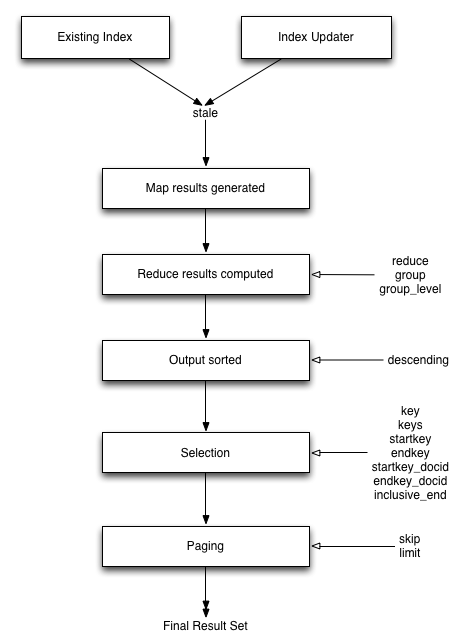
The core arguments and selection systems are the same through both the REST API interface, and the client libraries. The setting of these values differs between different client libraries, but the argument names and expected and supported values are the same across all environments.
Querying using the REST API
Querying can be performed through the REST API endpoint. The REST API supports and operates using the core HTTP protocol, and this is the same system used by the client libraries to obtain the view data.
For more information, see the REST API, Querying views.
Selecting information
Couchbase Server supports a number of mechanisms for selecting information returned by the view. Key selection is made after the view results (including the reduction function) are executed, and after the items in the view output have been sorted.
Important
When specifying keys to the selection mechanism, the key must be expressed in the form of a JSON value. For example, when specifying a single key, a string must be quoted ("string").When specifying the key selection through a parameter, the keys must match the format of the keys emitted by the view. Compound keys, for example where an array or hash has been used in the emitted key structure, the supplied selection value should also be an array or a hash.
The following selection types are supported:
-
Explicit Key
An explicit key can be specified using the parameter
key. The view query will only return results where the key in the view output, and the value supplied to thekeyparameter match identically.For example, if you supply the value “tomato” only records matching exactly “tomato” will be selected and returned. Keys with values such as “tomatoes” will not be returned.
-
Key List
A list of keys to be output can be specified by supplying an array of values using the
keysparameter. In this instance, each item in the specified array will be used as explicit match to the view result key, with each array value being combined with a logicalor.For example, if the value specified to the
keysparameter was["tomato","avocado"], then all results with a key of ‘tomato’ or ‘avocado’ will be returned.
Note
When using this query option, the output results are not sorted by key. This is because key sorting of these values would require collating and sorting all the rows before returning the requested information.
In the event of using a compound key, each compound key must be specified in the query. For example:
<pre><code class="no-highlight">keys=[["tomato",20],["avocado",20]]-
Key Range
A key range, consisting of a
startkeyandendkey. These options can be used individually, or together, as follows:-
startkeyonlyOutput does not start until the first occurrence of
startkey, or a value greater than the specified value, is seen. Output will then continue until the end of the view. -
endkeyonlyOutput starts with the first view result, and continues until the last occurrence of
endkey, or until the emitted value is greater than the computed lexical value ofendkey. -
startkeyandendkeyOutput of values does not start until
startkeyis seen, and stops when the last occurrence ofendkeyis identified.
When using
endkey, theinclusive_endoption specifies whether output stops after the last occurrence of the specifiedendkey(the default). If set to false, output stops on the last result before the specifiedendkeyis seen.The matching algorithm works on partial values, which can be used to an advantage when searching for ranges of keys. See Partial Selection and Key Ranges
-
Selecting compound information by key or keys
If you are generating a compound key within your view, for example when outputting a date split into individually year, month, day elements, then the selection value must exactly match the format and size of your compound key. The value of
keyorkeysmust exactly match the output key structure.For example, with the view data:
{"total_rows":5693,"rows":[
{"id":"1310653019.12667","key":[2011,7,14,14,16,59],"value":null},
{"id":"1310662045.29534","key":[2011,7,14,16,47,25],"value":null},
{"id":"1310668923.16667","key":[2011,7,14,18,42,3],"value":null},
{"id":"1310675373.9877","key":[2011,7,14,20,29,33],"value":null},
{"id":"1310684917.60772","key":[2011,7,14,23,8,37],"value":null},
{"id":"1310693478.30841","key":[2011,7,15,1,31,18],"value":null},
{"id":"1310694625.02857","key":[2011,7,15,1,50,25],"value":null},
{"id":"1310705375.53361","key":[2011,7,15,4,49,35],"value":null},
{"id":"1310715999.09958","key":[2011,7,15,7,46,39],"value":null},
{"id":"1310716023.73212","key":[2011,7,15,7,47,3],"value":null}
]
}
Using the
keyselection mechanism you must specify the entire key value, i.e.:?key=[2011,7,15,7,47,3]If you specify a value, such as only the date:
?key=[2011,7,15]The view will return no records, since there is no exact key match. Instead, you must use a range that encompasses the information range you want to output:
?startkey=[2011,7,15,0,0,0]&endkey=[2011,7,15,99,99,99]This will output all records within the specified range for the specified date. For more information, see Partial Selection with Compound Keys.
Partial selection and key ranges
Matching of the key value has a precedence from right to left for the key value and the supplied
startkeyand/orendkey. Partial strings may therefore be specified and return specific information.For example, given the view data:
"a",
 "aa",
 "bb",
 "bbb",
 "c",
 "cc",
 "ccc"
 "dddd"
Specifying a
startkeyparameter with the value “aa” will return the last seven records, including “aa”:"aa", "bb", "bbb", "c", "cc", "ccc", "dddd"Specifying a partial string to
startkeywill trigger output of the selected values as soon as the first value or value greater than the specified value is identified. For strings, this partial match (from left to right) is identified. For example, specifying astartkeyof “d” will return:"dddd"This is because the first match is identified as soon as the a key from a view row matches the supplied
startkeyvalue from left to right. The supplied single character matches the first character of the view output.When comparing larger strings and compound values the same matching algorithm is used. For example, searching a database of ingredients and specifying a
startkeyof “almond” will return all the ingredients, including “almond”, “almonds”, and “almond essence”.To match all of the records for a given word or value across the entire range, you can use the null value in the
endkeyparameter. For example, to search for all records that start only with the word “almond”, you specify astartkeyof “almond”, and an endkey of “almond\u02ad” (i.e. with the last Latin character at the end). If you are using Unicode strings, you may want to use “\uefff”.startkey="almond"&endkey="almond\u02ad"The precedence in this example is that output starts when ‘almond’ is seen, and stops when the emitted data is lexically greater than the supplied
endkey. Although a record with the value “almond\02ad” will never be seen, the emitted data will eventually be lexically greater than “almond\02ad” and output will stop.In effect, a range specified in this way acts as a prefix with all the data being output that match the specified prefix.
Partial selection with compound keys
Compound keys, such as arrays or hashes, can also be specified in the view output, and the matching precedence can be used to provide complex selection ranges. For example, if time data is emitted in the following format:
[year,month,day,hour,minute]Then precise date (and time) ranges can be selected by specifying the date and time in the generated data. For example, to get information between 1st April 2011, 00:00 and 30th September 2011, 23:59:
?startkey=[2011,4,1,0,0]&endkey=[2011,9,30,23,59]The flexible structure and nature of the
startkeyandendkeyvalues enable selection through a variety of range specifications. For example, you can obtain all of the data from the beginning of the year until the 5th March using:?startkey=[2011]&endkey=[2011,3,5,23,59]You can also examine data from a specific date through to the end of the month:
?startkey=[2011,3,16]&endkey=[2011,3,99]In the above example, the value for the
dayelement of the array is an impossible value, but the matching algorithm will identify when the emitted value is lexically greater than the suppliedendkeyvalue, and information selected for output will be stopped.A limitation of this structure is that it is not possible to ignore the earlier array values. For example, to select information from 10am to 2pm each day, you cannot use this parameter set:
?startkey=[null,null,null,10,0]&endkey=[null,null,null,14,0]In addition, because selection is made by a outputting a range of values based on the start and end key, you cannot specify range values for the date portion of the query:
?startkey=[0,0,0,10,0]&endkey=[9999,99,99,14,0]This will instead output all the values from the first day at 10am to the last day at 2pm.
For more information and examples on formatting and querying this data, see Date and Time Selection.
Pagination
Pagination over results can be achieved by using the
skipandlimitparameters. For example, to get the first 10 records from the view:?limit=10The next ten records can obtained by specifying:
?skip=10&limit=10On the server, the
skipoption works by executing the query and literally iterating over the specified number of output records specified byskip, then returning the remainder of the data up until the specifiedlimitrecords are reached, if thelimitparameter is specified.When paginating with larger values for
skip, the overhead for iterating over the records can be significant. A better solution is to track the document id output by the first query (with thelimitparameter). You can then usestartkey_docidto specify the last document ID seen, skip over that record, and output the next ten records.Therefore, the paging sequence is, for the first query:
?startkey="carrots"&limit=10Record the last document ID in the generated output, then use:
?startkey="carrots"&startkey_docid=DOCID&skip=1&limit=10When using
startkey_docidyou must specify thestartkeyparameter to specify the information being searched for. By using thestartkey_docidparameter, Couchbase Server skips through the B-Tree index to the specified document ID. This is much faster than the skip/limit example shown above.Grouping in queries
If you have specified an array as your compound key within your view, then you can specify the group level to be applied to the query output when using a
reduce().When grouping is enabled, the view output is grouped according to the key array, and you can specify the level within the defined array that the information is grouped by. You do this by specifying the index within the array by which you want the output grouped using the
group_levelparameter.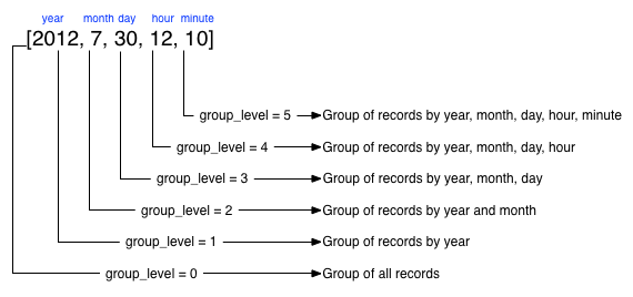
The
group_levelparameter specifies the array index (starting at 1) at which you want the grouping occur, and generate a unique value based on this value that is used to identify all the items in the view output that include this unique value:A group level of
0groups by the entire dataset (as if no array exists).A group level of
1groups the content by the unique value of the first element in the view key array. For example, when outputting a date split by year, month, day, hour, minute, each unique year will be output.A group level of
2groups the content by the unique value of the first and second elements in the array. With a date, this outputs each unique year and month, including all records with that year and month into each group.A group level of
3groups the content by the unique value of the first three elements of the view key array. In a date this outputs each unique date (year, month, day) grouping all items according to these first three elements.
The grouping will work for any output structure where you have output an compound key using an array as the output value for the key.
Selection when grouping
When using grouping and selection using the
key,keys, orstartkey/endkeyparameters, the query value should match at least the format (and element count) of the group level that is being queried.For example, using the following
map()function to output information by date as an array:function(doc, meta) { emit([doc.year, doc.mon, doc.day], doc.logtype); }If you specify a
group_levelof2then you must specify a key using at least the year and month information. For example, you can specify an explicit key, such as[2012,8]:?group=true&group_level=2&key=[2012,8]You can query it for a range:
?group=true&group_level=2&startkey=[2012,2]&endkey=[2012,8]You can also specify a year, month and day, while still grouping at a higher level. For example, to group by year/month while selecting by specific dates:
?group=true&group_level=2&startkey=[2012,2,15]&endkey=[2012,8,10]Specifying compound keys that are shorter than the specified group level may output unexpected results due to the selection mechanism and the way
startkeyandendkeyare used to start and stop the selection of output rows.Ordering
All view results are automatically output sorted, with the sorting based on the content of the key in the output view. Views are sorted using a specific sorting format, with the basic order for all basic and compound follows as follows:
nullfalsetrueNumbers
Text (case sensitive, lowercase first, UTF-8 order)
Arrays (according to the values of each element, in order)
Objects (according to the values of keys, in key order)
The natural sorting is therefore by default close to natural sorting order both alphabetically (A-Z) and numerically (0-9).
Note
There is no collation or foreign language support. Sorting is always according to the above rules based on UTF-8 values.
You can alter the direction of the sorting (reverse, highest to lowest numerically, Z-A alphabetically) by using the
descendingoption. When set to true, this reverses the order of the view results, ordered by their key.Because selection is made after sorting the view results, if you configure the results to be sorted in descending order and you are selecting information using a key range, then you must also reverse the
startkeyandendkeyparameters. For example, if you query ingredients where the start key is ‘tomato’ and the end key is ‘zucchini’, for example:?startkey="tomato"&endkey="zucchini"The selection will operate, returning information when the first key matches ‘tomato’ and stopping on the last key that matches ‘zucchini’.
If the return order is reversed:
?descending=true&startkey="tomato"&endkey="zucchini"The query will return only entries matching ‘tomato’. This is because the order will be reversed, ‘zucchini’ will appear first, and it is only when the results contain ‘tomato’ that any information is returned.
To get all the entries that match, the
startkeyandendkeyvalues must also be reversed:?descending=true&startkey="zucchini"&endkey="tomato"The above selection will start generating results when ‘zucchini’ is identified in the key, and stop returning results when ‘tomato’ is identified in the key.
Note
View output and selection are case sensitive. Specifying the key 'Apple' will not return 'apple' or 'APPLE' or other case differences. Normalizing the view output and query input to all lowercase or upper case will simplify the process by eliminating the case differences.
Understanding letter ordering in views
Couchbase Server uses a Unicode collation algorithm to order letters, so you should be aware of how this functions. Most developers are typically used to Byte order, such as that found in ASCII and which is used in most programming languages for ordering strings during string comparisons.
The following shows the order of precedence used in Byte order, such as ASCII:
123456890 < A-Z < a-zThis means any items that start with integers will appear before any items with letters; any items that beginning with capital letters will appear before items in lower case letters. This means the item named “Apple” will appear before “apple” and the item “Zebra” will appear before “apple”. Compare this with the order of precedence used in Unicode collation, which is used in Couchbase Server:
123456790 < aAbBcCdDeEfFgGhH...Notice again that items that start with integers will appear before any items with letters. However, in this case, the lowercase and then uppercase of the same letter are grouped together. This means that that if “apple” will appear before “Apple” and would also appear before “Zebra.” In addition, be aware that with accented characters will follow this ordering:
a < á < A < Á < bThis means that all items starting with “a” and accented variants of the letter will occur before “A” and any accented variants of “A.”
Ordering Example
In Byte order, keys in an index would appear as follows:
"ABC123" < "ABC223" < "abc123" < "abc223" < "abcd23" < "bbc123" < "bbcd23"The same items will be ordered this way by Couchbase Server under Unicode collation:
"abc123" < "ABC123" < "abc223" < "ABC223" < "abcd23" < "bbc123" < "bbcd23"This is particularly important for you to understand if you query Couchbase Server with a
startkeyandendkeyto get back a range of results. The items you would retrieve under Byte order are different compared to Unicode collation. For more information about ordering results, see Partial Selection and Key Ranges.Ordering and Query Example
This following example demonstrates Unicode collation in Couchbase Server and the impact on query results returned with a
startkeyandendkey. It is based on thebeer-sampledatabase provided with Couchbase Server. For more information, see Beer sample bucket.Imagine you want to retrieve all breweries with names starting with uppercase Y. Your query parameters would appear as follows:
startkey="Y"&endkey="z"If you want breweries starting with lowercase y or uppercase Y, you would provides a query as follows:
startkey="y"&endkey="z"This will return all names with lower case Y and items up to, but not including lowercase z, thereby including uppercase Y as well. To retrieve the names of breweries starting with lowercase y only, you would terminate your range with capital Y:
startkey="y"&endkey="Y"As it happens, the sample database does not contain any results because there are no beers in it which start with lowercase y. If you want to learn more about Unicode collation, refer to these resources: Unicode Technical Standard #10 and ICU User Guide, Customization, Default Options.
Error control
There are a number of parameters that can be used to help control errors and responses during a view query.
-
on_errorThe
on_errorparameter specifies whether the view results will be terminated on the first error from a node, or whether individual nodes can fail and other nodes return information.When returning the information generated by a view request, the default response is for any raised error to be included as part of the JSON response, but for the view process to continue. This allows for individual nodes within the Couchbase cluster to timeout or fail, while still generating the requested view information.
In this instance, the error is included as part of the JSON returned:
{
    "errors" : [
       {
          "from" : "http://192.168.1.80:9503/_view_merge/?stale=false",
          "reason" : "req_timedout"
       },
       {
          "from" : "http://192.168.1.80:9502/_view_merge/?stale=false",
          "reason" : "req_timedout"
       },
       {
          "from" : "http://192.168.1.80:9501/_view_merge/?stale=false",
          "reason" : "req_timedout"
       }
    ],
    "rows" : [
       {
          "value" : 333280,
          "key" : null
       }
    ]
 }
You can alter this behavior by using the
on_errorargument. The default value iscontinue. If you set this value tostopthen the view response will cease the moment an error occurs. The returned JSON will contain the error information for the node that returned the first error. For example:{ "errors" : [ { "from" : "http://192.168.1.80:9501/_view_merge/?stale=false", "reason" : "req_timedout" } ], "rows" : [ { "value" : 333280, "key" : null } ] }
View and query pattern samples
Building views and querying the indexes they generate is a combined process based both on the document structure and the view definition. Writing an effective view to query your data may require changing or altering your document structure, or creating a more complex view in order to allow the specific selection of the data through the querying mechanism.
For background and examples, the following selections provide a number of different scenarios and examples have been built to demonstrate the document structures, views and querying parameters required for different situations.
General advice
There are some general points and advice for writing all views that apply irrespective of the document structure, query format, or view content.
-
Do not assume the field will exist in all documents.
Fields may be missing from your document, or may only be supported in specific document types. Use an
iftest to identify problems. For example:if (document.firstname)… -
View output is case sensitive.
The value emitted by the
emit()function is case sensitive. Emitting a field value of ‘Martin’ but specifying akeyvalue of ‘martin’ will not match the data. Emitted data, and the key selection values, should be normalized to eliminate potential problems. For example:emit(doc.firstname.toLowerCase(),null); -
Number formatting
Numbers within JavaScript may inadvertently be converted and output as strings. To ensure that data is correctly formatted, the value should be explicitly converted. For example:
emit(parseInt(doc.value,10),null);The
parseInt()built-in function will convert a supplied value to an integer. TheparseFloat()function can be used for floating-point numbers.
Validating document type
If your dataset includes documents that may be either JSON or binary, then you do not want to create a view that outputs individual fields for non-JSON documents. You can fix this by using a view that checks the metadata
typefield before outputting the JSON view information:function(doc,meta) { if (meta.type == "json") { emit(doc.firstname.toLowerCase(),null); } }In the above example, the
emit()function will only be called on a valid JSON document. Non-JSON documents will be ignored and not included in the view output.Document ID (primary) index
To create a ‘primary key’ index, i.e. an index that contains a list of every document within the database, with the document ID as the key, you can create a simple view:
function(doc,meta)
{
  emit(meta.id,null);
}
This enables you to iterate over the documents stored in the database.
This will provide you with a view that outputs the document ID of every document in the bucket using the document ID as the key.
The view can be useful for obtaining groups or ranges of documents based on the document ID, for example to get documents with a specific ID prefix:
?startkey="object"&endkey="object\u0000"Or to obtain a list of objects within a given range:
?startkey="object100"&endkey="object199"Note
For all views, the document ID is automatically included as part of the view response. But the without including the document ID within the key emitted by the view, it cannot be used as a search or querying mechanism.
Secondary index
The simplest form of view is to create an index against a single field from the documents stored in your database.
For example, given the document structure:
{
    "firstname": "Martin",
    "lastname": "Brown"
}
A view to support queries on the
firstnamefield could be defined as follows:function(doc, meta) { if (doc.firstname) { emit(doc.firstname.toLowerCase(),null); } }The view works as follows for each document:
Only outputs a record if the document contains a
firstnamefield.Converts the content of the
firstnamefield to lowercase.
Queries can now be specified by supplying a string converted to lowercase. For example:
?key="martin"Will return all documents where the
firstnamefield contains ‘Martin’, regardless of the document field capitalization.Using expiration metadata
The metadata object makes it very easy to create and update different views on your data using information outside of the main document data. For example, you can use the expiration field within a view to get the list of recently active sessions in a system.
Using the following
map()function, which uses the expiration as part of the emitted data.function(doc, meta) { if (doc.type && doc.type == "session") { emit(meta.expiration, doc.nickname) } }If you have sessions which are saved with a TTL, this will allow you to give a view of who was recently active on the service.
Emitting multiple rows
The
emit()function is used to create a record of information for the view during the map phase, but it can be called multiple times within that map phase to allowing querying over more than one source of information from each stored document.An example of this is when the source documents contain an array of information. For example, within a recipe document, the list of ingredients is exposed as an array of objects. By iterating over the ingredients, an index of ingredients can be created and then used to find recipes by ingredient.
{
    "title": "Fried chilli potatoes",
    "preptime": "5"
    "servings": "4",
    "totaltime": "10",
    "subtitle": "A new way with chips.",
    "cooktime": "5",
    "ingredients": [
        {
            "ingredtext": "chilli powder",
            "ingredient": "chilli powder",
            "meastext": "3-6 tsp"
        },
        {
            "ingredtext": "potatoes, peeled and cut into wedges",
            "ingredient": "potatoes",
            "meastext": "900 g"
        },
        {
            "ingredtext": "vegetable oil for deep frying",
            "ingredient": "vegetable oil for deep frying",
            "meastext": ""
        }
    ],
}
The view can be created using the following
map()function:function(doc, meta) { if (doc.ingredients) { for (i=0; i < doc.ingredients.length; i++) { emit(doc.ingredients[i].ingredient, null); } } }To query for a specific ingredient, specify the ingredient as a key:
?key="carrot"The
keysparameter can also be used in this situation to look for recipes that contain multiple ingredients. For example, to look for recipes that contain either “potatoes” or “chilli powder” you would use:?keys=["potatoes","chilli powder"]This will produce a list of any document containing either ingredient. A simple count of the document IDs by the client can determine which recipes contain all three.
The output can also be combined. For example, to look for recipes that contain carrots and can be cooked in less than 20 minutes, the view can be rewritten as:
function(doc, meta) { if (doc.ingredients) { for (i=0; i < doc.ingredients.length; i++) { if (doc.ingredients[i].ingredtext && doc.totaltime) { emit([doc.ingredients[i].ingredtext, parseInt(doc.totaltime,10)], null); } } } }In this map function, an array is output that generates both the ingredient name, and the total cooking time for the recipe. To perform the original query, carrot recipes requiring less than 20 minutes to cook:
?startkey=["carrot",0]&endkey=["carrot",20]This generates the following view:
{"total_rows":26471,"rows":[
{"id":"Mangoandcarrotsmoothie","key":["carrots",5],"value":null},
{"id":"Cheeseandapplecoleslaw","key":["carrots",15],"value":null}
]
}
Date and time selection
For date and time selection, consideration must be given to how the data will need to be selected when retrieving the information. This is particularly true when you want to perform log roll-up or statistical collection by using a reduce function to count or quantify instances of a particular event over time.
Examples of this in action include querying data over a specific range, on specific day or date combinations, or specific time periods. Within a traditional relational database it is possible to perform an extraction of a specific date or date range by storing the information in the table as a date type.
Within a map/reduce, the effect can be simulated by exposing the date into the individual components at the level of detail that you require. For example, to obtain a report that counts individual log types over a period identifiable to individual days, you can use the following
map()function:function(doc, meta) { emit([doc.year, doc.mon, doc.day, doc.logtype], null); }By incorporating the full date into the key, the view provides the ability to search for specific dates and specific ranges. By modifying the view content you can simplify this process further. For example, if only searches by year/month are required for a specific application, the day can be omitted.
And with the corresponding
reduce()built-in of_count, you can perform a number of different queries. Without any form of data selection, for example, you can use thegroup_levelparameter to summarize down as far as individual day, month, and year. Additionally, because the date is explicitly output, information can be selected over a specific range, such as a specific month:endkey=[2010,9,30]&group_level=4&startkey=[2010,9,0]Here the explicit date has been specified as the start and end key. The
group_levelis required to specify roll-up by the date and log type.This will generate information similar to this:
{"rows":[
{"key":[2010,9,1,"error"],"value":5},
{"key":[2010,9,1,"warning"],"value":10},
{"key":[2010,9,2,"error"],"value":8},
{"key":[2010,9,2,"warning"],"value":9},
{"key":[2010,9,3,"error"],"value":16},
{"key":[2010,9,3,"warning"],"value":8},
{"key":[2010,9,4,"error"],"value":15},
{"key":[2010,9,4,"warning"],"value":11},
{"key":[2010,9,5,"error"],"value":6},
{"key":[2010,9,5,"warning"],"value":12}
]
}
Additional granularity, for example down to minutes or seconds, can be achieved by adding those as further arguments to the map function:
function(doc, meta)
{
    emit([doc.year, doc.mon, doc.day, doc.hour, doc.min, doc.logtype], null);
}
The same trick can also be used to output based on other criteria. For example, by day of the week, week number of the year or even by period:
function(doc, meta) {
  if (doc.mon)
  {
    var quarter = parseInt((doc.mon - 1)/3,10)+1;

    emit([doc.year, quarter, doc.logtype], null);
  }
}
To get more complex information, for example a count of individual log types for a given date, you can combine the
map()andreduce()stages to provide the collation.For example, by using the following
map()function we can output and collate by day, month, or year as before, and with data selection at the date level.function(doc, meta) { emit([doc.year, doc.mon, doc.day], doc.logtype); }For convenience, you may wish to use the
dateToArray()function, which converts a date object or string into an array. For example, if the date has been stored within the document as a single field:function(doc, meta) { emit(dateToArray(doc.date), doc.logtype); }For more information, see
dateToArray().Using the following
reduce()function, data can be collated for each individual logtype for each day within a single record of output.function(key, values, rereduce) { var response = {"warning" : 0, "error": 0, "fatal" : 0 }; for(i=0; i<values.length; i++) { if (rereduce) { response.warning = response.warning + values[i].warning; response.error = response.error + values[i].error; response.fatal = response.fatal + values[i].fatal; } else { if (values[i] == "warning") { response.warning++; } if (values[i] == "error" ) { response.error++; } if (values[i] == "fatal" ) { response.fatal++; } } } return response; }When queried using a
group_levelof two (by month), the following output is produced:{"rows":[ {"key":[2010,7], "value":{"warning":4,"error":2,"fatal":0}}, {"key":[2010,8], "value":{"warning":4,"error":3,"fatal":0}}, {"key":[2010,9], "value":{"warning":4,"error":6,"fatal":0}}, {"key":[2010,10],"value":{"warning":7,"error":6,"fatal":0}}, {"key":[2010,11],"value":{"warning":5,"error":8,"fatal":0}}, {"key":[2010,12],"value":{"warning":2,"error":2,"fatal":0}}, {"key":[2011,1], "value":{"warning":5,"error":1,"fatal":0}}, {"key":[2011,2], "value":{"warning":3,"error":5,"fatal":0}}, {"key":[2011,3], "value":{"warning":4,"error":4,"fatal":0}}, {"key":[2011,4], "value":{"warning":3,"error":6,"fatal":0}} ] }The input includes a count for each of the error types for each month. Note that because the key output includes the year, month and date, the view also supports explicit querying while still supporting grouping and roll-up across the specified group. For example, to show information from 15th November 2010 to 30th April 2011 using the following query:
?endkey=[2011,4,30]&group_level=2&startkey=[2010,11,15]Which generates the following output:
{"rows":[
{"key":[2010,11],"value":{"warning":1,"error":8,"fatal":0}},
{"key":[2010,12],"value":{"warning":3,"error":4,"fatal":0}},
{"key":[2011,1],"value":{"warning":8,"error":2,"fatal":0}},
{"key":[2011,2],"value":{"warning":4,"error":7,"fatal":0}},
{"key":[2011,3],"value":{"warning":4,"error":4,"fatal":0}},
{"key":[2011,4],"value":{"warning":5,"error":7,"fatal":0}}
]
}
Note
Keep in mind that you can create multiple views to provide different views and queries on your document data. In the above example, you could create individual views for the limited data types of logtype to create a
warningsbydateview.Selective record output
If you are storing different document types within the same bucket, then you may want to ensure that you generate views only on a specific record type within the
map()phase. This can be achieved by using anifstatement to select the record.For example, if you are storing blog ‘posts’ and ‘comments’ within the same bucket, then a view on the blog posts could be created using the following map:
function(doc, meta) {
    if (doc.title && doc.type && doc.date &&
        doc.author && doc.type == 'post')
    {
        emit(doc.title, [doc.date, doc.author]);
    }
}
The same solution can also be used if you want to create a view over a specific range or value of documents while still allowing specific querying structures. For example, to filter all the records from the statistics logging system over a date range that are of the type error you could use the following
map()function:function(doc, meta) { if (doc.logtype == 'error') { emit([doc.year, doc.mon, doc.day],null); } }The same solution can also be used for specific complex query types. For example, all the recipes that can be cooked in under 30 minutes, made with a specific ingredient:
function(doc, meta) { if (doc.totaltime && doc.totaltime <= 20) { if (doc.ingredients) { for (i=0; i < doc.ingredients.length; i++) { if (doc.ingredients[i].ingredtext) { emit(doc.ingredients[i].ingredtext, null); } } } } }The above function allows for much quicker and simpler selection of recipes by using a query and the
keyparameter, instead of having to work out the range that may be required to select recipes when the cooking time and ingredients are generated by the view.These selections are application specific, but by producing different views for a range of appropriate values, for example 30, 60, or 90 minutes, recipe selection can be much easier at the expense of updating additional view indexes.
Sorting on reduce values
The sorting algorithm within the view system outputs information ordered by the generated key within the view, and therefore it operates before any reduction takes place. Unfortunately, it is not possible to sort the output order of the view on computed reduce values, as there is no post-processing on the generated view information.
To sort based on reduce values, you must access the view content with reduction enabled from a client, and perform the sorting within the client application.
Solutions for simulating joins
Joins between data, even when the documents being examined are contained within the same bucket, are not possible directly within the view system. However, you can simulate this by making use of a common field used for linking when outputting the view information. For example, consider a blog post system that supports two different record types, ‘blogpost’ and ‘blogcomment’. The basic format for ‘blogpost’ is:
{
    "type" : "post",
    "title" : "Blog post"
    "categories" : [...],
    "author" : "Blog author"
    ...
}
The corresponding comment record includes the blog post ID within the document structure:
{
    "type" : "comment",
    "post_id" : "post_3454"
    "author" : "Comment author",
    "created_at" : 123498235
...
}
To output a blog post and all the comment records that relate to the blog post, you can use the following view:
function(doc, meta)
{
    if (doc.post_id && doc.type && doc.type == "post")
    {
        emit([doc.post_id, null], null);
    }
    else if (doc.post_id && doc.created_at && doc.type && doc.type == "comment")
    {
        emit([doc.post_id, doc.created_at], null);
    }
}
The view makes use of the sorting algorithm when using arrays as the view key. For a blog post record, the document ID will be output will a null second value in the array, and the blog post record will therefore appear first in the sorted output from the view. For a comment record, the first value will be the blog post ID, which will cause it to be sorted in line with the corresponding parent post record, while the second value of the array is the date the comment was created, allowing sorting of the child comments.
For example:
{"rows":[
{"key":["post_219",null],       "value":{...}},
{"key":["post_219",1239875435],"value":{...}},
{"key":["post_219",1239875467],"value":{...}},
]
}
Another alternative is to make use of a multi-get operation within your client through the main Couchbase SDK interface, which should load the data from cache. This allows you to structure your data with the blog post containing an array of the of the child comment records. For example, the blog post structure might be:
{
    "type" : "post",
    "title" : "Blog post"
    "categories" : [...],
    "author" : "Blog author",
    "comments": ["comment_2298","comment_457","comment_4857"],
    ...
}
To obtain the blog post information and the corresponding comments, create a view to find the blog post record, and then make a second call within your client SDK to get all the comment records from the Couchbase Server cache.
Simulating transactions
Couchbase Server does not support transactions, but the effect can be simulated by writing a suitable document and view definition that produces the effect while still only requiring a single document update to be applied.
For example, consider a typical banking application, the document structure could be as follows:
{
   "account" : "James",
   "value" : 100
}
A corresponding record for another account:
{
   "account" : "Alice",
   "value" : 200
}
To get the balance of each account, the following
map():function(doc, meta) { if (doc.account && doc.value) { emit(doc.account,doc.value); } }The
reduce()function can use the built-in_sumfunction.When queried, using a
group_levelof 1, the balance of the accounts is displayed:{"rows":[ {"key":"Alice","value":200}, {"key":"James","value":100} ] }Money in an account can be updated just by adding another record into the system with the account name and value. For example, adding the record:
{
   "account" : "James",
   "value" : 50
}
Re-querying the view produces an updated balance for each account:
{"rows":[
{"key":"Alice","value":200},
{"key":"James","value":150}
]
}
However, if Alice wants to transfer $100 to James, two record updates are required:
A record that records an update to Alice’s account to reduce the value by 100.
A record that records an update to James’s account to increase the value by 100.
Unfortunately, the integrity of the transaction could be compromised in the event of a problem between step 1 and step 2. Alice’s account may be deducted, without updates James' record.
To simulate this operation while creating (or updating) only one record, a combination of a transaction record and a view must be used. The transaction record looks like this:
{
     "fromacct" : "Alice",
     "toacct" : "James",
     "value" : 100
}
The above records the movement of money from one account to another. The view can now be updated to handle a transaction record and output a row through
emit()to update the value for each account.function(doc, meta) { if (doc.fromacct) { emit(doc.fromacct, -doc.value); emit(doc.toacct, doc.value); } else { emit(doc.account, doc.value); } }The above
map()effectively generates two fake rows, one row subtracts the amount from the source account, and adds the amount to the destination account. The resulting view then uses thereduce()function to sum up the transaction records for each account to arrive at a final balance:{"rows":[ {"key":"Alice","value":100}, {"key":"James","value":250} ] }Throughout the process, only one record has been created, and therefore transient problems with that record update can be captured without corrupting or upsetting the existing stored data.
Simulating multi-phase transactions
The technique in Simulating Transactions will work if your data will allow the use of a view to effectively roll-up the changes into a single operation. However, if your data and document structure do not allow it then you can use a multi-phase transaction process to perform the operation in a number of distinct stages.
Warning
This method is not reliant on views, but the document structure and update make it easy to find out if there are 'hanging' or trailing transactions that need to be processed without additional document updates. Using views and the
observeoperation to monitor changes could lead to long wait times during the transaction process while the view index is updated.To employ this method, you use a similar transaction record as in the previous example, but use the transaction record to record each stage of the update process.
Start with the same two account records:
{
   "type" : "account",
   "account" : "James",
   "value" : 100,
   "transactions" : []
}
The record explicitly contains a
transactionsfield which contains an array of all the currently active transactions on this record.The corresponding record for the other account:
{
   "type" : "account",
   "account" : "Alice",
   "value" : 200,
   "transactions" : []
}
Now perform the following operations in sequence:
-
Create a new transaction record that records the transaction information:
{
      "type" : "transaction",
      "fromacct" : "Alice",
      "toacct" : "James",
      "value" : 100,
      "status" : "waiting"
 }
The core of the transaction record is the same, the difference is the use of a
statusfield which will be used to monitor the progress of the transaction.Record the ID of the transaction, for example,
transact_20120717163. -
Set the value of the
statusfield in the transaction document to ‘pending’:{ "type" : "transaction", "fromacct" : "Alice", "toacct" : "James", "value" : 100, "status" : "pending" } -
Find all transaction records in the
pendingstate using a suitable view:function(doc, meta) { if (doc.type && doc.status && doc.type == "transaction" && doc.status == "pending" ) { emit([doc.fromacct,doc.toacct], doc.value); } } -
Update the record identified in
toacctwith the transaction information, ensuring that the transaction is not already pending:{ "type" : "account", "account" : "Alice", "value" : 100, "transactions" : ["transact_20120717163"] }Repeat on the other account:
{ "type" : "account", "account" : "James", "value" : 200, "transactions" : ["transact_20120717163"] } -
Update the transaction record to mark that the records have been updated:
{ "type" : "transaction", "fromacct" : "Alice", "toacct" : "James", "value" : 100, "status" : "committed" } -
Find all transaction records in the
committedstate using a suitable view:function(doc, meta) { if (doc.type && doc.status && doc.type == "transaction" && doc.status == "committed" ) { emit([doc.fromacct, doc.toacct], doc.value); } }Update the source account record noted in the transaction and remove the transaction ID:
{
      "type" : "account",
      "account" : "Alice",
      "value" : 100,
      "transactions" : []
   }
Repeat on the other account:
{
      "type" : "account",
      "account" : "James",
      "value" : 200,
      "transactions" : []
   }
Update the transaction record state to ‘done’. This will remove the transaction from the two views used to identify unapplied, or uncommitted transactions.
Within this process, although there are multiple steps required, you can identify at each step whether a particular operation has taken place or not.
For example, if the transaction record is marked as ‘pending’, but the corresponding account records do not contain the transaction ID, then the record still needs to be updated. Since the account record can be updated using a single atomic operation, it is easy to determine if the record has been updated or not.
The result is that any sweep process that accesses the views defined in each step can determine whether the record needs updating. Equally, if an operation fails, a record of the transaction, and whether the update operation has been applied, also exists, allowing the changes to be reversed and backed out.
Translating SQL to map/reduce
SELECT fieldlist FROM table \
    WHERE condition \
    GROUP BY groupfield \
    ORDER BY orderfield \
    LIMIT limitcount OFFSET offsetcount
The different elements within the source statement affect how a view is written in the following ways:
-
SELECT fieldlistThe field list within the SQL statement affects either the corresponding key or value within the
map()function, depending on whether you are also selecting or reducing your data. See Translating SQL Field Selection (SELECT) to Map/Reduce -
FROM tableThere are no table compartments within Couchbase Server and you cannot perform views across more than one bucket boundary. However, if you are using a
typefield within your documents to identify different record types, then you may want to use themap()function to make a selection.For examples of this in action, see Selective Record Output.
-
WHERE conditionThe
map()function and the data generated into the view key directly affect how you can query, and therefore how selection of records takes place. For examples of this in action, see Translating SQL WHERE to Map/Reduce. -
ORDER BY orderfieldThe order of record output within a view is directly controlled by the key specified during the
map()function phase of the view generation.For further discussion, see Translating SQL ORDER BY to Map/Reduce.
-
LIMIT limitcount OFFSET offsetcountThere are a number of different paging strategies available within the map/reduce and views mechanism. Discussion on the direct parameters can be seen in Translating SQL LIMIT and OFFSET. For alternative paging solutions, see Pagination.
-
GROUP BY groupfieldGrouping within SQL is handled within views through the use of the
reduce()function. For comparison examples, see Translating SQL GROUP BY to Map/Reduce.
The interaction between the view
map()function,reduce()function, selection parameters and other miscellaneous parameters according to the table below:SQL Statement Fragment View Key View Value map()Functionreduce()FunctionSelection Parameters Other Parameters SELECT fields Yes Yes Yes No: with GROUP BYandSUM()orCOUNT()functions onlyNo No FROM table No No Yes No No No WHERE clause Yes No Yes No Yes No ORDER BY field Yes No Yes No No descendingLIMIT x OFFSET y No No No No No limit,skipGROUP BY field Yes Yes Yes Yes No No Within SQL, the basic query structure can be used for a multitude of different queries. For example, the same ‘
SELECT fieldlist FROM table WHERE xxxxcan be used with a number of different clauses.Within map/reduce and Couchbase Server, multiple views may be needed to be created to handled different query types. For example, performing a query on all the blog posts on a specific date will need a very different view definition than one needed to support selection by the author.
Translating SQL SELECT to map/reduce
The field selection within an SQL query can be translated into a corresponding view definition, either by adding the fields to the emitted key (if the value is also used for selection in a
WHEREclause), or into the emitted value, if the data is separate from the required query parameters.For example, to get the sales data by country from each stored document using the following
map()function:function(doc, meta) { emit([doc.city, doc.sales], null); }If you want to output information that can be used within a reduce function, this should be specified in the value generated by each
emit()call. For example, to reduce the sales figures the abovemap()function could be rewritten as:function(doc, meta) { emit(doc.city, doc.sales); }In essence this does not produce significantly different output (albeit with a simplified key), but the information can now be reduced using the numerical value.
If you want to output data or field values completely separate to the query values, then these fields can be explicitly output within the value portion of the view. For example:
function(doc, meta) {
  emit(doc.city, [doc.name, doc.sales]);
}
If the entire document for each item is required, load the document data after the view has been requested through the client library. For more information on this parameter and the performance impact, see View Writing Best Practice.
Note
Within a
SELECTstatement it is common practice to include the primary key for a given record in the output. Within a view this is not normally required, since the document ID that generated each row is always included within the view output.Translating SQL WHERE to map/reduce
The
WHEREclause within an SQL statement forms the selection criteria for choosing individual records. Within a view, the ability to query the data is controlled by the content and structure of thekeygenerated by themap()function.In general, for each
WHEREclause you need to include the corresponding field in the key of the generated view, and then use thekey,keysorstartkey/endkeycombinations to indicate the data you want to select.. The complexity occurs when you need to perform queries on multiple fields. There are a number of different strategies that you can use for this.The simplest way is to decide whether you want to be able to select a specific combination, or whether you want to perform range or multiple selections. For example, using our recipe database, if you want to select recipes that use the ingredient ‘carrot’ and have a cooking time of exactly 20 minutes, then you can specify these two fields in the
map()function:function(doc, meta) { if (doc.ingredients) { for(i=0; i < doc.ingredients.length; i++) { emit([doc.ingredients[i].ingredient, doc.totaltime], null); } } }Then the query is an array of the two selection values:
?key=["carrot",20]This is equivalent to the SQL query:
SELECT recipeid FROM recipe JOIN ingredients on ingredients.recipeid = recipe.recipeid
    WHERE ingredient = 'carrot' AND totaltime = 20
If, however, you want to perform a query that selects recipes containing carrots that can be prepared in less than 20 minutes, a range query is possible with the same
map()function:?startkey=["carrot",0]&endkey=["carrot",20]This works because of the sorting mechanism in a view, which outputs in the information sequentially, fortunately nicely sorted with carrots first and a sequential number.
More complex queries though are more difficult. What if you want to select recipes with carrots and rice, still preparable in under 20 minutes?
A standard
map()function like that above wont work. A range query on both ingredients will list all the ingredients between the two. There are a number of solutions available to you. First, the easiest way to handle the timing selection is to create a view that explicitly selects recipes prepared within the specified time. I.E:function(doc, meta) { if (doc.totaltime <= 20) { ... } }Although this approach seems to severely limit your queries, remember you can create multiple views, so you could create one for 10 mins, one for 20, one for 30, or whatever intervals you select. It’s unlikely that anyone will really want to select recipes that can be prepared in 17 minutes, so such granular selection is overkill.
The multiple ingredients is more difficult to solve. One way is to use the client to perform two queries and merge the data. For example, the
map()function:function(doc, meta) { if (doc.totaltime && doc.totaltime <= 20) { if (doc.ingredients) { for(i=0; i < doc.ingredients.length; i++) { emit(doc.ingredients[i].ingredient, null); } } } }Two queries, one for each ingredient can easily be merged by performing a comparison and count on the document ID output by each view.
The alternative is to output the ingredients twice within a nested loop, like this:
function(doc, meta) { if (doc.totaltime && doc.totaltime <= 20) { if (doc.ingredients) { for (i=0; i < doc.ingredients.length; i++) { for (j=0; j < doc.ingredients.length; j++) { emit([doc.ingredients[i].ingredient, doc.ingredients[j].ingredient], null); } } } } }Now you can perform an explicit query on both ingredients:
?key=["carrot","rice"]If you really want to support flexible cooking times, then you can also add the cooking time:
function(doc, meta)
{
  if (doc.ingredients)
  {
    for (i=0; i < doc.ingredients.length; i++)
    {
      for (j=0; j < doc.ingredients.length; j++)
      {
        emit([doc.ingredients[i].ingredient, doc.ingredients[j].ingredient, recipe.totaltime], null);
      }
    }
  }
}
And now you can support a ranged query on the cooking time with the two ingredient selection:
?startkey=["carrot","rice",0]&key=["carrot","rice",20]This would be equivalent to:
SELECT recipeid FROM recipe JOIN ingredients on ingredients.recipeid = recipe.recipeid
    WHERE (ingredient = 'carrot' OR ingredient = 'rice') AND totaltime = 20
Translating SQL ORDER BY to map/reduce
The
ORDER BYclause within SQL controls the order of the records that are output. Ordering within a view is controlled by the value of the key. However, the key also controls and supports the querying mechanism.In
SELECTstatements where there is no explicitWHEREclause, the emitted key can entirely support the sorting you want. For example, to sort by the city and salesman name, the followingmap()will achieve the required sorting:function(doc, meta) { emit([doc.city, doc.name], null) }If you need to query on a value, and that query specification is part of the order sequence then you can use the format above. For example, if the query basis is city, then you can extract all the records for ‘London’ using the above view and a suitable range query:
?endkey=["London\u0fff"]&startkey=["London"]However, if you want to query the view by the salesman name, you need to reverse the field order in the
emit()statement:function(doc, meta) { emit([doc.name,doc.city],null) }Now you can search for a name while still getting the information in city order.
The order the output can be reversed (equivalent to
ORDER BY field DESC) by using thedescendingquery parameter. For more information, see Ordering.Translating SQL GROUP BY to map/reduce
The
GROUP BYparameter within SQL provides summary information for a group of matching records according to the specified fields, often for use with a numeric field for a sum or total value, or count operation.For example:
SELECT name,city,SUM(sales) FROM sales GROUP BY name,cityThis query groups the information by the two fields ‘name’ and ‘city’ and produces a sum total of these values. To translate this into a map/reduce function within Couchbase Server:
From the list of selected fields, identify the field used for the calculation. These will need to be exposed within the value emitted by the
map()function.Identify the list of fields in the
GROUP BYclause. These will need to be output within the key of themap()function.Identify the grouping function, for example
SUM()orCOUNT(). You will need to use the equivalent built-in function, or a custom function, within thereduce()function of the view.
For example, in the above case, the corresponding map function can be written as
map():function(doc, meta) { emit([doc.name,doc.city],doc.sales); }This outputs the name and city as the key, and the sales as the value. Because the
SUM()function is used, the built-inreduce()function_sumcan be used.An example of this map/reduce combination can be seen in Built-in _sum.
More complex grouping operations may require a custom reduce function. For more information, see Writing Custom Reduce Functions.
Translating SQL LIMIT and OFFSET
Within SQL, the
LIMITandOFFSETclauses to a given query are used as a paging mechanism. For example, you might use:SELECT recipeid,title FROM recipes LIMIT 100To get the first 100 rows from the database, and then use the
OFFSETto get the subsequent groups of records:SELECT recipeid,title FROM recipes LIMIT 100 OFFSET 100With Couchbase Server, the
limitandskipparameters when supplied to the query provide the same basic functionality:?limit=100&skip=100Performance for high values of skip can be affected. See Pagination for some further examples of paging strategies.
Writing geospatial views
Geospatial support was introduced as an experimental feature in Couchbase Server. This feature is currently unsupported and is provided only for the purposes of demonstration and testing.
GeoCouch adds two-dimensional spatial index support to Couchbase. Spatial support enables you to record geometry data into the bucket and then perform queries which return information based on whether the recorded geometries existing within a given two-dimensional range such as a bounding box. This can be used in spatial queries and in particular geolocationary queries where you want to find entries based on your location or region.
The GeoCouch support is provided through updated index support and modifications to the view engine to provide advanced geospatial queries.
Adding geometry data
GeoCouch supports the storage of any geometry information using the GeoJSON specification. The format of the storage of the point data is arbitrary with the geometry type being supported during the view index generation.
For example, you can use two-dimensional geometries for storing simple location data. You can add these to your Couchbase documents using any field name. The convention is to use a single field with two-element array with the point location, but you can also use two separate fields or compound structures as it is the view that compiles the information into the geospatial index.
For example, to populate a bucket with city location information, the document sent to the bucket could be formatted like that below:
{
"loc" : [-122.270833, 37.804444],
"title" : "Oakland"
}
Views and queries
The GeoCouch extension uses the standard Couchbase indexing system to build a two-dimensional index from the point data within the bucket. The format of the index information is based on the GeoJSON specification.
To create a geospatial index, use the
emit()function to output a GeoJSON Point value containing the coordinates of the point you are describing. For example, the following function will create a geospatial index on the earlier spatial record example.function(doc, meta) { if (doc.loc) { emit( { type: "Point", coordinates: doc.loc, }, [meta.id, doc.loc]); } }The key in the spatial view index can be any valid GeoJSON geometry value, including points, multipoints, linestrings, polygons and geometry collections.
The view
map()function should be placed into a design document using thespatialprefix to indicate the nature of the view definition. For example, the following design document includes the above function as the viewpoints{ "spatial" : { "points" : "function(doc, meta) { if (doc.loc) { emit({ type: \"Point\", coordinates: [doc.loc[0], doc.loc[1]]}, [meta.id, doc.loc]);}}", } }To execute the geospatial query you use the design document format using the embedded spatial indexing. For example, if the design document is called
mainwithin the bucketplaces, the URL will behttp://localhost:8092/places/_design/main/_spatial/points.Spatial queries include support for a number of additional arguments to the view request. The full list is provided in the following summary table.
Get Spatial Name Description Method GET /bucket/_design/design-doc/_spatial/spatial-nameRequest Data None Response Data JSON of the documents returned by the view Authentication Required no Query Arguments bboxSpecify the bounding box for a spatial query Parameters : string; optional limitLimit the number of the returned documents to the specified number Parameters : numeric; optional skipSkip this number of records before starting to return the results Parameters : numeric; optional staleAllow the results from a stale view to be used Parameters : string; optional Supported Values false: Force update of the view index before results are returnedok: Allow stale viewsupdate_after: Allow stale view, update view after accessBounding Box Queries If you do not supply a bounding box, the full dataset is returned. When querying a spatial index you can use the bounding box to specify the boundaries of the query lookup on a given value. The specification should be in the form of a comma-separated list of the coordinates to use during the query.
These coordinates are specified using the GeoJSON format, so the first two numbers are the lower left coordinates, and the last two numbers are the upper right coordinates.
For example, using the above design document:
GET http://localhost:8092/places/_design/main/_spatial/points?bbox=0,0,180,90
Content-Type: application/json
Returns the following information:
{
   "update_seq" : 3,
   "rows" : [
      {
         "value" : [
            "oakland",
            [
               10.898333,
               48.371667
            ]
         ],
         "bbox" : [
            10.898333,
            48.371667,
            10.898333,
            48.371667
         ],
         "id" : "augsburg"
      }
   ]
}
Note that the return data includes the value specified in the design document view function, and the bounding box of each individual matching document. If the spatial index includes the
bboxbounding box property as part of the specification, then this information will be output in place of the automatically calculated version.Monitoring Couchbase
There are a number of different ways in which you can monitor Couchbase. You should be aware however of some of the basic issues that you will need to know before starting your monitoring procedure.
Underlying server processes
There are several different server processes that constantly run in Couchbase Server whether or not the server is actively handling reads/writes or handling other operations from a client application. Right after you start up a node, you may notice a spike in CPU utilization, and the utilization rate will plateau at some level greater than zero. The following describes the ongoing processes that are running on your node:
-
beam.smp on Linux: erl.exe on Windows
These processes are responsible for monitoring and managing all other underlying server processes such as ongoing XDCR replications, cluster operations, and views.
There is a separate monitoring/babysitting process running on each node. The process is small and simple and therefore unlikely to crash due to lack of memory. It is responsible for spawning and monitoring the second, larger process for cluster management, XDCR and views. It also spawns and monitors the processes for Moxi and memcached. If any of these three processes fail, the monitoring process will re-spawn them.
The main benefit of this approach is that an Erlang VM crash will not cause the Moxi and memcached processes to also crash. You will also see two
beam.smporerl.exeprocesses running on Linux or Windows respectively.The set of log files for this monitoring process is
ns_server.babysitter.logwhich you can collect withcbcollect_info. See the cbcollect_info tool. memcached : This process is responsible for caching items in RAM and persisting them to disk.
moxi : This process enables third-party memcached clients to connect to the server.
Port numbers and accessing different buckets
In a Couchbase Server cluster, any communication (stats or data) to a port other than 11210 will result in the request going through a Moxi process. This means that any stats request will be aggregated across the cluster (and may produce some inconsistencies or confusion when looking at stats that are not “aggregatable”).
In general, it is best to run all your stat commands against port 11210 which will always give you the information for the specific node that you are sending the request to. It is a best practice to then aggregate the relevant data across nodes at a higher level (in your own script or monitoring system).
When you run the below commands (and all stats commands) without supplying a bucket name and/or password, they will return results for the default bucket and produce an error if one does not exist.
To access a bucket other than the default, you will need to supply the bucket name and/or password on the end of the command. Any bucket created on a dedicated port does not require a password.
Warning
The TCP/IP port allocation on Windows by default includes a restricted number of ports available for client communication. For more information on this issue, including information on how to adjust the configuration and increase the available ports, see MSDN: Avoiding TCP/IP Port Exhaustion.
Monitoring startup (warmup)
If a Couchbase Server node is starting up for the first time, it will create whatever DB files necessary and begin serving data immediately. However, if there is already data on disk (likely because the node rebooted or the service restarted) the node needs to read all of this data off of disk before it can begin serving data. This is called “warmup”. Depending on the size of data, this can take some time. For more information about server warmup, see Handling Server Warmup.
When starting up a node, there are a few statistics to monitor. Use the
cbstatscommand to watch the warmup and item stats:> cbstats localhost:11210 -b bucket_name -p bucket_password warmup | » egrep "warm|curr_items"curr_items: 0 curr_items_tot: 15687 ep_warmed_up: 15687 ep_warmup: false ep_warmup_dups: 0 ep_warmup_oom: 0 ep_warmup_thread: running ep_warmup_time: 787 And when it is complete:
> cbstats localhost:11210 -b bucket_name -p bucket_password warmup | »
    egrep "warm|curr_items"
curr_items: 10000 curr_items_tot: 20000 ep_warmed_up: 20000 ep_warmup: true ep_warmup_dups: 0 ep_warmup_oom: 0 ep_warmup_thread: complete ep_warmup_time 1400 Stat Description curr_items The number of items currently active on this node. During warmup, this will be 0 until complete curr_items_tot The total number of items this node knows about (active and replica). During warmup, this will be increasing and should match ep_warmed_up ep_warmed_up The number of items retrieved from disk. During warmup, this should be increasing. ep_warmup_dups The number of duplicate items found on disk. Ideally should be 0, but a few is not a problem ep_warmup_oom How many times the warmup process received an Out of Memory response from the server while loading data into RAM ep_warmup_thread The status of the warmup thread. Can be either running or complete ep_warmup_time How long the warmup thread was running for. During warmup this number should be increasing, when complete it will tell you how long the process took Disk write queue
Couchbase Server is a persistent database which means that part of monitoring the system is understanding how we interact with the disk subsystem.
Since Couchbase Server is an asynchronous system, any mutation operation is committed first to DRAM and then queued to be written to disk. The client is returned an acknowledgment almost immediately so that it can continue working. There is replication involved here too, but we’re ignoring it for the purposes of this discussion.
We have implemented disk writing as a 2-queue system and they are tracked by the stats. The first queue is where mutations are immediately placed. Whenever there are items in that queue, our “flusher” (disk writer) comes along and takes all the items off of that queue, places them into the other one and begins writing to disk. Since disk performance is so dramatically different than RAM, this allows us to continue accepting new writes while we are (possibly slowly) writing new ones to the disk.
The flusher will process 250k items a a time, then perform a disk commit and continue this cycle until its queue is drained. When it has completed everything in its queue, it will either grab the next group from the first queue or essentially sleep until there are more items to write.
Monitoring the disk write queue
There are basically two ways to monitor the disk queue, at a high-level from the Web UI or at a low-level from the individual node statistics.
- From the Web UI, click on Monitor Data Buckets and select the particular bucket that you want to monitor.
- Click “Configure View” in the top right corner and select the “Disk Write Queue” statistic. Closing this window shows that there is a new mini-graph.
This graph is showing the Disk Write Queue for all nodes in the cluster. To get a deeper view into this statistic, you can monitor each node individually using the ‘stats’ output (see Viewing Server Nodes for more information about gathering node-level stats). There are two statistics to watch here:
ep_queue_size (where new mutations are placed) flusher_todo (the queue of items currently being written to disk)
See The Dispatcher for more information about monitoring what the disk subsystem is doing at any given time.
Couchbase Server statistics
Couchbase Server provides statistics at multiple levels throughout the cluster. These are used for regular monitoring, capacity planning and to identify the performance characteristics of your cluster deployment. The most visible statistics are those in the Web UI, but components such as the REST interface, the proxy and individual nodes have directly accessible statistics interfaces.
REST interface statistics
To interact with statistics provided by REST, use the Couchbase Web Console. This GUI gathers statistics via REST and displays them to your browser. The REST interface has a set of resources that provide access to the current and historic statistics the cluster gathers and stores. See the REST API for more information.
Couchbase Server node statistics
Detailed stats documentation can be found in the repository.
Along with stats at the REST and UI level, individual nodes can also be queried for statistics either through a client which uses binary protocol or through the cbstats utility shipped with Couchbase Server.
For example:
> cbstats localhost:11210 all
 auth_cmds:                   9
 auth_errors:                 0
 bucket_conns:                10
 bytes_read:                  246378222
 bytes_written:               289715944
 cas_badval:                  0
 cas_hits:                    0
 cas_misses:                  0
 cmd_flush:                   0
 cmd_get:                     134250
 cmd_set:                     115750
…
The most commonly needed statistics are surfaced through the Web Console and have descriptions there and in the associated documentation. Software developers and system administrators wanting lower level information have it available through the stats interface.
There are seven commands available through the stats interface:
stats(referred to as ‘all’)dispatcherhashtaptimingsvkeyreset
stats command
This displays a large list of statistics related to the Couchbase process including the underlying engine (ep_* stats).
dispatcher command
This statistic will show what the dispatcher is currently doing:
dispatcher
     runtime: 45ms
       state: dispatcher_running
      status: running
        task: Running a flusher loop.
nio_dispatcher
       state: dispatcher_running
      status: idle
The first entry, dispatcher, monitors the process responsible for disk access. The second entry is a non-IO (non disk) dispatcher. There may also be a ro_dispatcher dispatcher present if the engine is allowing concurrent reads and writes. When a task is actually running on a given dispatcher, the “runtime” tells you how long the current task has been running. Newer versions will show you a log of recently run dispatcher jobs so you can see what’s been happening.
Changing statistics collection
The default Couchbase Server statistics collection is set to collect every second. The tuning that is available for statistic collection is by collecting statistics less frequently.
Note
If statistic collection is changed from the default, the Couchbase service must be restarted.
To change statistic collection:
- Log in as root or sudo and navigate to the directory where Couchbase is installed. For example:
/opt/couchbase/etc/couchbase/static_config - Edit the static_config file.
- Add the following parameter: {grab_stats_every_n_ticks, 10}, where 10 is the number of ticks. In the Couchbase environment one tick is one second (default). It is recommended that the statistics collection be more frequent (and accurate). However, assign an appropriate tick value for you environment.
- Restart the Couchbase service.
After restarting the Couchbase service, the statistics collection rate will be changed.
Changing the stats file location
The default stats file location is
/opt/couchbase/var/lib/couchbase/stats, however, if you want to change the default stats file location, create a symlink location to the new directory.Note
When creating a symlink, stop and restart the Couchbase service.
Couchbase Server Moxi statistics
Moxi, as part of it’s support of memcached protocol, has support for the memcached
statscommand. Regular memcached clients can request statistics through the memcached stats command. The stats command accepts optional arguments, and in the case of Moxi, there is a stats proxy sub-command. A detailed description of statistics available through Moxi can be found in the Moxi 1.8 Manual.For example, one simple client one may use is the commonly available netcat (output elided with ellipses):
$ echo "stats proxy" | nc localhost 11211
STAT basic:version 1.6.0
STAT basic:nthreads 5
…
STAT proxy_main:conf_type dynamic
STAT proxy_main:behavior:cycle 0
STAT proxy_main:behavior:downstream_max 4
STAT proxy_main:behavior:downstream_conn_max 0
STAT proxy_main:behavior:downstream_weight 0
…
STAT proxy_main:stats:stat_configs 1
STAT proxy_main:stats:stat_config_fails 0
STAT proxy_main:stats:stat_proxy_starts 2
STAT proxy_main:stats:stat_proxy_start_fails 0
STAT proxy_main:stats:stat_proxy_existings 0
STAT proxy_main:stats:stat_proxy_shutdowns 0
STAT 11211:default:info:port 11211
STAT 11211:default:info:name default
…
STAT 11211:default:behavior:downstream_protocol 8
STAT 11211:default:behavior:downstream_timeout 0
STAT 11211:default:behavior:wait_queue_timeout 0
STAT 11211:default:behavior:time_stats 0
STAT 11211:default:behavior:connect_max_errors 0
STAT 11211:default:behavior:connect_retry_interval 0
STAT 11211:default:behavior:front_cache_max 200
STAT 11211:default:behavior:front_cache_lifespan 0
STAT 11211:default:behavior:front_cache_spec
STAT 11211:default:behavior:front_cache_unspec
STAT 11211:default:behavior:key_stats_max
STAT 11211:default:behavior:key_stats_lifespan 0
STAT 11211:default:behavior:key_stats_spec
STAT 11211:default:behavior:key_stats_unspec
STAT 11211:default:behavior:optimize_set
STAT 11211:default:behavior:usr default
…
STAT 11211:default:pstd_stats:num_upstream 1
STAT 11211:default:pstd_stats:tot_upstream 2
STAT 11211:default:pstd_stats:num_downstream_conn 1
STAT 11211:default:pstd_stats:tot_downstream_conn 1
STAT 11211:default:pstd_stats:tot_downstream_conn_acquired 1
STAT 11211:default:pstd_stats:tot_downstream_conn_released 1
STAT 11211:default:pstd_stats:tot_downstream_released 2
STAT 11211:default:pstd_stats:tot_downstream_reserved 1
STAT 11211:default:pstd_stats:tot_downstream_reserved_time 0
STAT 11211:default:pstd_stats:max_downstream_reserved_time 0
STAT 11211:default:pstd_stats:tot_downstream_freed 0
STAT 11211:default:pstd_stats:tot_downstream_quit_server 0
STAT 11211:default:pstd_stats:tot_downstream_max_reached 0
STAT 11211:default:pstd_stats:tot_downstream_create_failed 0
STAT 11211:default:pstd_stats:tot_downstream_connect 1
STAT 11211:default:pstd_stats:tot_downstream_connect_failed 0
STAT 11211:default:pstd_stats:tot_downstream_connect_timeout 0
STAT 11211:default:pstd_stats:tot_downstream_connect_interval 0
STAT 11211:default:pstd_stats:tot_downstream_connect_max_reached 0
…
END
Troubleshooting
When troubleshooting your Couchbase Server deployment there are a number of different approaches available to you. For specific answers to individual problems, see Common Errors.
General tips
The following are some general tips that may be useful before performing any more detailed investigations:
Try pinging the node.
Try connecting to the Couchbase Server Web Console on the node.
Try to use
telnetto connect to the various ports that Couchbase Server uses.Try reloading the web page.
Check firewall settings (if any) on the node. Make sure there isn’t a firewall between you and the node. On a Windows system, for example, the Windows firewall might be blocking the ports (Control Panel > Windows Firewall).
Make sure that the documented ports are open between nodes and make sure the data operation ports are available to clients.
Check your browser’s security settings.
Check any other security software installed on your system, such as antivirus programs.
-
Generate a Diagnostic Report for use by Couchbase Technical Support to help determine what the problem is. There are two ways of collecting this information:
Click
Generate Diagnostic Reporton the Log page to obtain a snapshot of your system’s configuration and log information for deeper analysis. You must send this file to Couchbase.-
Run the
cbcollect_infoon each node within your cluster. To run, you must specify the name of the file to be generated:> cbcollect_info nodename.zipThis will create a Zip file with the specified name. You must run each command individually on each node within the cluster. You can then send each file to Couchbase for analysis.
For more information, see the cbcollect_info tool.
Responding to specific errors
The following table outlines some specific areas to check when experiencing different problems:
Severity Issue Suggested Action(s) Critical Couchbase Server does not start up. Check that the service is running. Check error logs. Try restarting the service. Critical A server is not responding. Check that the service is running. Check error logs. Try restarting the service. Critical A server is down. Try restarting the server. Use the command-line interface to check connectivity. Informational Bucket authentication failure. Check the properties of the bucket that you are attempting to connect to. The primary source for run-time logging information is the Couchbase Server Web Console. Run-time logs are automatically set up and started during the installation process. However, the Couchbase Server gives you access to lower-level logging details if needed for diagnostic and troubleshooting purposes. Log files are stored in a binary format in the logs directory under the Couchbase installation directory. You must use
browse_logsto extract the log contents from the binary format to a text file.Logs and logging
Couchbase Server creates a number of different log files depending on the component of the system that produce the error, and the level and severity of the problem being reported. For a list of the different file locations for each platform, see .
Platform Location Linux /opt/couchbase/var/lib/couchbase/logsWindows C:\Program Files\Couchbase\Server\var\lib\couchbase\logsAssumes default installation locationMac OS X /Users/couchbase/Library/Application Support/Couchbase/var/lib/couchbase/logsIndividual log files are automatically numbered, with the number suffix incremented for each new log, with a maximum of 20 files per log. Individual log file sizes are limited to 10MB by default.
The following table contains a list of the different log files are create in the logging directory and their contents.
File Log Contents couchdbErrors relating to the couchdb subsystem that supports views, indexes and related REST API issues debugDebug level error messages related to the core server management subsystem, excluding information included in the couchdb,xdcrandstatslogs.infoInformation level error messages related to the core server management subsystem, excluding information included in the couchdb,xdcrandstatslogs.http_access.logThe admin access log records server requests (including admin logins) coming through the REST or Couchbase web console. It is output in common log format and contains several important fields such as remote client IP, timestamp, GET/POST request and resource requested, HTTP status code, and so on. errorError level messages for all subsystems excluding xdcr.xcdr_errorXDCR error messages. xdcrXDCR information messages. tmpfailFor XDCR, the destination cluster is not able to eject items fast enough to make room for new mutations. XDCR retries several times, without throwing errors, but after a fixed number of attempts the errors are shown to the user. Nevertheless, if a user waits long enough, XDCR eventually retries and is able to replicate the remaining data. mapreduce_errorsJavaScript and other view-processing errors are reported in this file. viewsErrors relating to the integration between the view system and the core server subsystem. statsContains periodic reports of the core statistics. memcached.logContains information relating to the core memcache component, including vBucket and replica and rebalance data streams requests. reports.logContains only progress report and crash reports for the Erlang process. Note
Each log file group will also include a
.idxand.sizfile which holds meta information about the log file group. These files are automatically updated by the logging system.Changing log file location
The default file log location is /opt/couchbase/var/lib/couchbase/logs, however, if you want to change the default log location to a different directory, change the log file configuration option.
Note
To implement a log file location change (from the default), you must be log in as either root or sudo and the Couchbase service must be restarted.
To change the log file configuration:
- Log in as root or sudo and navigate to the directory where you installed Couchbase. For example:
/opt/couchbase/etc/couchbase/static_config - Edit the static_config file and change the
error_logger_mf_dirvariable to a different directory. For example:{error_logger_mf_dir, "/home/user/cb/opt/couchbase/var/lib/couchbase/logs"} - Restart the Couchbase service. After restarting the Couchbase service, all subsequent logs will be in the new directory.
Changing logging levels
The default logging level for all log files are set to debug except for couchdb, which is set to info. If you want to change the default logging level, modify the logging level configuration options.
The configuration change can be performed in one of the following ways:
- persistent
- dynamic (on the fly, without restarting).
Changing logging levels to be persistent
Logging levels can be changed so that the changes are persistent, that is, the changes continue to be implemented should a Couchbase Server reboot occur.
Note
To implement logging level changes, the Couchbase service must be restarted.
To change logging levels to be persistent:
- Log in as root or sudo and navigate to the directory where you installed Couchbase. For example:
/opt/couchbase/etc/couchbase/static_config - Edit the static_config file and change the desired log component. For example, parameters with the
loglevel_prefix set the logging level. - Restart the Couchbase service.
After restarting the Couchbase service, logging levels for that component will be changed.
Changing logging levels dynamically
If logging levels are changed dynamically and if a Couchbase server reboot occurs, then the changed logging levels revert to the default.
To change logging levels dynamically, execute a curl POST command using the following syntax:
curl -X POST -u adminName:adminPassword HOST:PORT/diag/eval –d ‘ale:set_loglevel(<log_component>,<logging_level>).’- Where:
- Log_component
- The default log level (except couchdb) is debug. For example, ns_server. The available loggers are ns_server, couchdb, user, Menelaus, ns_doctor, stats, rebalance, cluster, views, mapreduce_errors , xdcr and error_logger
- Logging_level
- The available log levels are debug, info, warning, and error.
Example
curl -X POST -u Administrator:password
  http://127.0.0.1:8091/diag/eval
  -d 'ale:set_loglevel(ns_server,error).
Changing the log rotation settings
Each log group is rotated automatically, by default storing 20 files of 10MB each. The log rotation settings can be changed by modifying the logging configuration in
/opt/couchbase/etc/couchbase/static_config.Note
To change the log rotation settings, log in as either root or sudo and restart the Couchbase service.
To change the log file configuration:
- Log in as root or sudo and navigate to the directory where you installed Couchbase. For example:
/opt/couchbase/etc/couchbase/static_config - Edit the static_config file and change the
error_logger_mf_maxfilesanderror_logger_mf_maxbytesvariables to the desired values. For example:{error_logger_mf_maxbytes, 20971520}.and{error_logger_mf_maxfiles, 40}.gives 40 files of 20MB each. - Stop the Couchbase service.
- Either delete or move all the files from the log directory (default location is
/opt/couchbase/var/lib/couchbase/logs) - Start the Couchbase service.
After starting the Couchbase service, all subsequent logs are rotated using the new values.
Common errors
This page will attempt to describe and resolve some common errors that are encountered when using Couchbase. It will be a living document as new problems and/or resolutions are discovered.
-
Problems Starting Couchbase Server for the first time
If you are having problems starting Couchbase Server on Linux for the first time, there are two very common causes of this that are actually quite related. When the
/etc/init.d/couchbase-serverscript runs, it tries to set the file descriptor limit and core file size limit:> ulimit -n 10240 ulimit -c unlimitedDepending on the defaults of your system, this may or may not be allowed. If Couchbase Server is failing to start, you can look through the logs and pick out one or both of these messages:
ns_log: logging ns_port_server:0:Port server memcached on node ‘ns_1@127.0.0.1’ exited with status 71. »
  Restarting. Messages: failed to set rlimit for open files. »
  Try running as root or requesting smaller maxconns value.
Alternatively, you may additionally see or optionally see:
ns_port_server:0:info:message - Port server memcached on node ‘ns_1@127.0.0.1’ exited with status 71. »
  Restarting. Messages: failed to ensure corefile creation
The resolution to these is to edit the /etc/security/limits.conf file and add these entries:
couchbase hard nofile 10240
  couchbase hard core unlimited
Troubleshooting views
A number of errors and problems with views are generally associated with the eventual consistency model of the view system. In this section, some further detail on this information and strategies for identifying and tracking view errors are provided.
It also gives some guidelines about how to report potential view engine issues, what information to include in JIRA.
Timeout errors in query responses
When querying a view with
stale=false, you get often timeout errors for one or more nodes. These nodes are nodes that did not receive the original query request, for example you query node 1, and you get timeout errors for nodes 2, 3 and 4 as in the example below (view with reduce function _count):> curl -s 'http://localhost:9500/default/_design/dev_test2/_view/view2?full_set=true&stale=false' {"rows":[ {"key":null,"value":125184} ], "errors":[ {"from":"http://192.168.1.80:9503/_view_merge/?stale=false","reason":"timeout"}, {"from":"http://192.168.1.80:9501/_view_merge/?stale=false","reason":"timeout"}, {"from":"http://192.168.1.80:9502/_view_merge/?stale=false","reason":"timeout"} ] }The problem here is that by default, for queries with
stale=false(full consistency), the view merging node (node which receive the query request, node 1 in this example) waits up to 60000 milliseconds (1 minute) to receive partial view results from each other node in the cluster. If it waits for more than 1 minute for results from a remote node, it stops waiting for results from that node and a timeout error entry is added to the final response. Astale=falserequest blocks a client, or the view merger node as in this example, until the index is up to date, so these timeouts can happen frequently.If you look at the logs from those nodes you got a timeout error, you’ll see the index build/update took more than 60 seconds, example from node 2:
[couchdb:info,2012-08-20T15:21:13.150,n_1@192.168.1.80:<0.6234.0>:couch_log:info:39] Set view
  `default`, main group `_design/dev_test2`, updater finished
 Indexing time: 93.734 seconds
 Blocked time:  10.040 seconds
 Inserted IDs:  124960
 Deleted IDs:   0
 Inserted KVs:  374880
 Deleted KVs:   0
 Cleaned KVs:   0
In this case, node 2 took 103.774 seconds to update the index.
In order to avoid those timeouts, you can pass a large connection_timeout in the view query URL, example:
> time curl -s
 'http://localhost:9500/default/_design/dev_test2/_view/view2?full_set=true&stale=false&connection_timeout=999999999'
{"rows":[
{"key":null,"value":2000000}
]
}
real  2m44.867s
user   0m0.007s
sys    0m0.007s
And in the logs of nodes 1, 2, 3 and 4, respectively you’ll see something like this:
node 1, view merger node[couchdb:info,2012-08-20T16:10:02.887,n_0@192.168.1.80:<0.27674.0>:couch_log:info:39] Set view `default`, main group `_design/dev_test2`, updater finished Indexing time: 155.549 seconds Blocked time: 0.000 seconds Inserted IDs:96 Deleted IDs: 0 Inserted KVs: 1500288 Deleted KVs: 0 Cleaned KVs: 0node 2[couchdb:info,2012-08-20T16:10:28.457,n_1@192.168.1.80:<0.6071.0>:couch_log:info:39] Set view `default`, main group `_design/dev_test2`, updater finished Indexing time: 163.555 seconds Blocked time: 0.000 seconds Inserted IDs: 499968 Deleted IDs: 0 Inserted KVs: 1499904 Deleted KVs: 0 Cleaned KVs: 0node 3[couchdb:info,2012-08-20T16:10:29.710,n_2@192.168.1.80:<0.6063.0>:couch_log:info:39] Set view `default`, main group `_design/dev_test2`, updater finished Indexing time: 164.808 seconds Blocked time: 0.000 seconds Inserted IDs: 499968 Deleted IDs: 0 Inserted KVs: 1499904 Deleted KVs: 0 Cleaned KVs: 0node 4[couchdb:info,2012-08-20T16:10:26.686,n_3@192.168.1.80:<0.6063.0>:couch_log:info:39] Set view `default`, main group `_design/dev_test2`, updater finished Indexing time: 161.786 seconds Blocked time: 0.000 seconds Inserted IDs: 499968 Deleted IDs: 0 Inserted KVs: 1499904 Deleted KVs: 0 Cleaned KVs: 0Blocked indexers, no progress for long periods of time
Each design document maps to one indexer, so when the indexer runs it updates all views defined in the corresponding design document. Indexing takes resources (CPU, disk IO, memory), therefore Couchbase Server limits the maximum number of indexers that can run in parallel. There are 2 configuration parameters to specify the limit, one for regular (main/active) indexers and other for replica indexers (more on this in a later section). The default for the former is 4 and for the later is 2. They can be queried like this:
> curl -s 'http://Administrator:asdasd@localhost:8091/settings/maxParallelIndexers' {"globalValue":4,"nodes":{"n_0@192.168.1.80":4}}maxParallelIndexersis for main indexes andmaxParallelReplicaIndexersis for replica indexes. When there are more design documents (indexers) than maxParallelIndexers, some indexers are blocked until there’s a free slot, and the rule is simple as first-come-first-served. These slots are controlled by 2 barriers processes, one for main indexes, and the other for replica indexes. Their current state can be seen from_active_tasks(per node), for example when there’s no indexing happening:> curl -s 'http://localhost:9500/_active_tasks' | json_xs [ { "waiting" : 0, "started_on" : 1345642656, "pid" : "<0.234.0>", "type" : "couch_main_index_barrier", "running" : 0, "limit" : 4, "updated_on" : 1345642656 }, { "waiting" : 0, "started_on" : 1345642656, "pid" : "<0.235.0>", "type" : "couch_replica_index_barrier", "running" : 0, "limit" : 2, "updated_on" : 1345642656 } ]The
waitingfields tells us how many indexers are blocked, waiting for their turn to run. Queries withstale=falsehave to wait for the indexer to be started (if not already), unblocked and to finish, which can lead to a long time when there are many design documents in the system. Also take into account that the indexer for a particular design document might be running for one node but it might be blocked in another node - when it’s blocked it’s not necessarily blocked in all nodes of the cluster nor when it’s running is necessarily running in all nodes of the cluster - you verify this by querying _active_tasks for each node (this API is not meant for direct user consumption, just for developers and debugging/troubleshooting).Through
_active_tasks(remember, it’s per node, so check it for every node in the cluster), you can see which indexers are running and which are blocked. Here follows an example where we have 5 design documents (indexers) and>maxParallelIndexersis 4:> curl -s 'http://localhost:9500/_active_tasks' | json_xs [ { "waiting" : 1, "started_on" : 1345644651, "pid" : "<0.234.0>", "type" : "couch_main_index_barrier", "running" : 4, "limit" : 4, "updated_on" : 1345644923 }, { "waiting" : 0, "started_on" : 1345644651, "pid" : "<0.235.0>", "type" : "couch_replica_index_barrier", "running" : 0, "limit" : 2, "updated_on" : 1345644651 }, { "indexer_type" : "main", "started_on" : 1345644923, "updated_on" : 1345644923, "design_documents" : [ "_design/test" ], "pid" : "<0.4706.0>", "signature" : "4995c136d926bdaf94fbe183dbf5d5aa", "type" : "blocked_indexer", "set" : "default" }, { "indexer_type" : "main", "started_on" : 1345644923, "progress" : 0, "initial_build" : true, "updated_on" : 1345644923, "total_changes" : 250000, "design_documents" : [ "_design/test4" ], "pid" : "<0.4715.0>", "changes_done" : 0, "signature" : "15e1f576bc85e3e321e28dc883c90077", "type" : "indexer", "set" : "default" }, { "indexer_type" : "main", "started_on" : 1345644923, "progress" : 0, "initial_build" : true, "updated_on" : 1345644923, "total_changes" : 250000, "design_documents" : [ "_design/test3" ], "pid" : "<0.4719.0>", "changes_done" : 0, "signature" : "018b83ca22e53e14d723ea858ba97168", "type" : "indexer", "set" : "default" }, { "indexer_type" : "main", "started_on" : 1345644923, "progress" : 0, "initial_build" : true, "updated_on" : 1345644923, "total_changes" : 250000, "design_documents" : [ "_design/test2" ], "pid" : "<0.4722.0>", "changes_done" : 0, "signature" : "440b0b3ded9d68abb559d58b9fda3e0a", "type" : "indexer", "set" : "default" }, { "indexer_type" : "main", "started_on" : 1345644923, "progress" : 0, "initial_build" : true, "updated_on" : 1345644923, "total_changes" : 250000, "design_documents" : [ "_design/test7" ], "pid" : "<0.4725.0>", "changes_done" : 0, "signature" : "fd2bdf6191e61af6e801e3137e2f1102", "type" : "indexer", "set" : "default" } ]The indexer for design document _design/test is represented by a task with a
typefield ofblocked_indexer, while other indexers have a task with typeindexer, meaning they’re running. The task with typecouch_main_index_barrierconfirms this by telling us there are currently 4 indexers running and 1 waiting for its turn. When an indexer is allowed to execute, its active task with typeblocked_indexeris replaced by a new one with typeindexer.Data missing in query response or it’s wrong (user issue)
For example, you defined a view with a
_statsreduce function. You query your view, and keep getting empty results all the time, for example:> curl -s 'http://localhost:9500/default/_design/dev_test3/_view/view1?full_set=true' {"rows":[ ] }You repeat this query over and over for several minutes or even hours, and you always get an empty result set.
Try to query the view with
stale=false, and you get:> curl -s 'http://localhost:9500/default/_design/dev_test3/_view/view1?full_set=true&stale=false' {"rows":[ ], "errors":[ {"from":"local","reason":"Builtin _stats function requires map values to be numbers"}, {"from":"http://192.168.1.80:9502/_view_merge/?stale=false","reason":"Builtin _stats function requires map values to be numbers"}, {"from":"http://192.168.1.80:9501/_view_merge/?stale=false","reason":"Builtin _stats function requires map values to be numbers"}, {"from":"http://192.168.1.80:9503/_view_merge/?stale=false","reason":"Builtin _stats function requires map values to be numbers"} ] }Then looking at the design document, you see it could never work, as values are not numbers:
{
   "views":
   {
       "view1": {
           "map": "function(doc, meta) { emit(meta.id, meta.id); }",
           "reduce": "_stats"
       }
   }
}
One important question to answer is, why do you see the errors when querying with
stale=falsebut do not see them when querying withstale=update_after(default) orstale=ok? The answer is simple:stale=falsemeans: trigger an index update/build, and wait until it that update/build finishes, then start streaming the view results. For this example, index build/update failed, so the client gets an error, describing why it failed, from all nodes where it failed.stale=update_aftermeans start streaming the index contents immediately and after trigger an index update (if index is not up to date already), so query responses won’t see indexing errors as they do for thestale=falsescenario. For this particular example, the error happened during the initial index build, so the index was empty when the view queries arrived in the system, whence the empty result set.stale=okis very similar to (2), except it doesn’t trigger index updates.
Finally, index build/update errors, related to user Map/Reduce functions, can be found in a dedicated log file that exists per node and has a file name matching
mapreduce_errors.#. For example, from node 1, the file*mapreduce_errors.1contained:[mapreduce_errors:error,2012-08-20T16:18:36.250,n_0@192.168.1.80:<0.2096.1>] Bucket `default`, main group `_design/dev_test3`, error executing reduce function for view `view1' reason: Builtin _stats function requires map values to be numbersWrong documents or rows when querying with include_docs=true
Imagine you have the following design document:
{
     "meta": {"id": "_design/test"},
     "views":
     {
         "view1": {
             "map": "function(doc, meta) { emit(meta.id,  doc.value); }"
         }
     }
 }
And the bucket only has 2 documents, document
doc1with JSON value{"value": 1}, and documentdoc2with JSON value{"value": 2}, you query the view initially withstale=falseandinclude_docs=trueand get:> curl -s 'http://localhost:9500/default/_design/test/_view/view1?include_docs=true&stale=false' | json_xs { "total_rows" : 2, "rows" : [ { "value" : 1, "doc" : { "json" : { "value" : 1 }, "meta" : { "flags" : 0, "expiration" : 0, "rev" : "1-000000367916708a0000000000000000", "id" : "doc1" } }, "id" : "doc1", "key" : "doc1" }, { "value" : 2, "doc" : { "json" : { "value" : 2 }, "meta" : { "flags" : 0, "expiration" : 0, "rev" : "1-00000037b8a32e420000000000000000", "id" : "doc2" } }, "id" : "doc2", "key" : "doc2" } ] }Later on you update both documents, such that document
doc1has the JSON value{"value": 111111}and documentdoc2has the JSON value{"value": 222222}. You then query the view withstale=update_after(default) orstale=okand get:> curl -s 'http://localhost:9500/default/_design/test/_view/view1?include_docs=true' | json_xs { "total_rows" : 2, "rows" : [ { "value" : 1, "doc" : { "json" : { "value" : 111111 }, "meta" : { "flags" : 0, "expiration" : 0, "rev" : "2-0000006657aeed6e0000000000000000", "id" : "doc1" } }, "id" : "doc1", "key" : "doc1" }, { "value" : 2, "doc" : { "json" : { "value" : 222222 }, "meta" : { "flags" : 0, "expiration" : 0, "rev" : "2-00000067e3ee42620000000000000000", "id" : "doc2" } }, "id" : "doc2", "key" : "doc2" } ] }The documents included in each row don’t match the value field of each row, that is, the documents included are the latest (updated) versions but the index row values still reflect the previous (first) version of the documents.
Why this behavior? Well,
include_docs=trueworks at query time, for each row, to fetch from disk the latest revision of each document. There’s no way to include a previous revision of a document. Previous revisions are not accessible through the latest vbucket databases MVCC snapshots ( http://en.wikipedia.org/wiki/Multiversion_concurrency_control ), and it’s not possible to find efficiently from which previous MVCC snapshots of a vbucket database a specific revision of a document is located. Further, vbucket database compaction removes all previous MVCC snapshots (document revisions). In short, this is a deliberate design limit of the database engine.The only way to ensure full consistency here is to include the documents themselves in the values emitted by the map function. Queries with
stale=falseare not 100% reliable either, as just after the index is updated and while rows are being streamed from disk to the client, document updates and deletes can still happen, resulting in the same behavior as in the given example.Expired documents still have their associated key-value pairs returned in queries with stale=false
See http://www.couchbase.com/issues/browse/MB-6219
Data missing in query response or it’s wrong (potentially due to server issues)
Sometimes, especially between releases for development builds, it’s possible results are missing due to issues in some component of Couchbase Server. This section describes how to do some debugging to identify which components, or at least to identify which components are not at fault.
Before proceeding, it needs to be mentioned that each vbucket is physically represented by a CouchDB database (generated by couchstore component) which corresponds to exactly 1 file in the filesystem, example from a development environment using 16 vbuckets only (for example simplicity), 4 nodes and without replicas enabled:
> tree ns_server/couch/0/
ns_server/couch/0/
 ???
_replicator.couch.1
 ???
_users.couch.1
 ??? default
     ??? 0.couch.1
     ??? 1.couch.1
     ??? 2.couch.1
     ??? 3.couch.1
     ??? master.couch.1
     ??? stats.json

 1 directory, 8 files

> tree ns_server/couch/1/
ns_server/couch/1/
 ???
_replicator.couch.1
 ???
_users.couch.1
 ??? default
     ??? 4.couch.1
     ??? 5.couch.1
     ??? 6.couch.1
     ??? 7.couch.1
     ??? master.couch.1
     ??? stats.json
     ??? stats.json.old

 1 directory, 9 files

> tree ns_server/couch/2/
ns_server/couch/2/
 ???
_replicator.couch.1
 ???
_users.couch.1
 ??? default
     ??? 10.couch.1
     ??? 11.couch.1
     ??? 8.couch.1
     ??? 9.couch.1
     ??? master.couch.1
     ??? stats.json
     ??? stats.json.old

 1 directory, 9 files

> tree ns_server/couch/3/
ns_server/couch/3/
 ???
_replicator.couch.1
 ???
_users.couch.1
 ??? default
     ??? 12.couch.1
     ??? 13.couch.1
     ??? 14.couch.1
     ??? 15.couch.1
     ??? master.couch.1
     ??? stats.json
     ??? stats.json.old

 1 directory, 9 files
For this particular example, because there are
no replicas enabled(ran./cluster_connect -n 4 -r 0), each node only has database files for the vbuckets it’s responsible for (active vbuckets). The numeric suffix in each database filename, starts at 1 when the database file is created and it gets incremented, by 1, every time the vbucket is compacted. If replication is enabled, for example you ran./cluster_connect -n 4 -r 1, then each node will have vbucket database files for the vbuckets it’s responsible for (active vbuckets) and for some replica vbuckets, example:> tree ns_server/couch/0/ ns_server/couch/0/ ??? _replicator.couch.1 ??? _users.couch.1 ??? default ??? 0.couch.1 ??? 1.couch.1 ??? 12.couch.1 ??? 2.couch.1 ??? 3.couch.1 ??? 4.couch.1 ??? 5.couch.1 ??? 8.couch.1 ??? master.couch.1 ??? stats.json 1 directory, 12 files > tree ns_server/couch/1/ ns_server/couch/1/ ??? _replicator.couch.1 ??? _users.couch.1 ??? default ??? 0.couch.1 ??? 1.couch.1 ??? 13.couch.1 ??? 4.couch.1 ??? 5.couch.1 ??? 6.couch.1 ??? 7.couch.1 ??? 9.couch.1 ??? master.couch.1 ??? stats.json 1 directory, 12 files > tree ns_server/couch/2/ ns_server/couch/2/ ??? _replicator.couch.1 ??? _users.couch.1 ??? default ??? 10.couch.1 ??? 11.couch.1 ??? 14.couch.1 ??? 15.couch.1 ??? 2.couch.1 ??? 6.couch.1 ??? 8.couch.1 ??? 9.couch.1 ??? master.couch.1 ??? stats.json 1 directory, 12 files > tree ns_server/couch/3/ ns_server/couch/3/ ??? _replicator.couch.1 ??? _users.couch.1 ??? default ??? 10.couch.1 ??? 11.couch.1 ??? 12.couch.1 ??? 13.couch.1 ??? 14.couch.1 ??? 15.couch.1 ??? 3.couch.1 ??? 7.couch.1 ??? master.couch.1 ??? stats.json 1 directory, 12 filesYou can figure out which vbucket are active in each node, by querying the following URL:
> curl -s http://localhost:8091/pools/default/buckets |
  json_xs
 [
    {
       "quota" :
{
          "rawRAM" : 268435456,
          "ram"
: 1073741824
       },
       "localRandomKeyUri" : "/pools/default/buckets/default/localRandomKey",
       "bucketCapabilitiesVer" : "",
       "authType"
: "sasl",
       "uuid" :
  "89dd5c64504f4a9414a2d3bcf9630d15",
       "replicaNumber" : 1,
       "vBucketServerMap" : {
          "vBucketMap" : [
             [
                0,
                1
             ],
             [
                0,
                1
             ],
             [
                0,
                2
             ],
             [
                0,
                3
             ],
             [
                1,
                0
             ],
             [
                1,
                0
             ],
             [
                1,
                2
             ],
             [
                1,
                3
             ],
             [
                2,
                0
             ],
             [
                2,
                1
             ],
             [
                2,
                3
             ],
             [
                2,
                3
             ],
             [
                3,
                0
             ],
             [
                3,
                1
             ],
             [
                3,
                2
             ],
             [
                3,
                2
             ]
          ],
          "numReplicas" : 1,
          "hashAlgorithm" : "CRC",
          "serverList" : [
             "192.168.1.81:12000",
             "192.168.1.82:12002",
             "192.168.1.83:12004",
             "192.168.1.84:12006"
          ]
       },

(....)
 ]
The field to look at is named
vBucketServerMap, and it contains two important sub-fields, namedvBucketMapandserverList, which we use to find out which nodes are responsible for which vbuckets (active vbuckets).Looking at these 2 fields, we can do the following active and replica vbucket to node mapping:
vbuckets 0, 1, 2 and 3 are active at node 192.168.1.81:12000, and vbuckets 4, 5, 8 and 12 are replicas at that same node
vbuckets 4, 5, 6 and 7 are active at node 192.168.1.82:12002, and vbuckets 0, 1, 9 and 13 are replicas at that same node
vbuckets 8, 9, 10 and 11 are active at node 192.168.1.83:12004, and vbuckets 2, 6, 14 and 15 are replicas at that same node
vbuckets 12, 13, 14 and 15 are active at node 192.168.1.84:12006, and vbucket 3, 7, 11 and 10
the value of
vBucketMapis an array of arrays of 2 elements. Each sub-array corresponds to a vbucket, so the first one is related to vbucket 0, second one to vbucket 1, etc, and the last one to vbucket 15. Each sub-array element is an index (starting at 0) into theserverListarray. First element of each sub-array tells us which node (server) has the corresponding vbucket marked as active, while the second element tells us which server has this vbucket marked as replica.If the replication factor is greater than 1 (N > 1), then each sub-array will have N + 1 elements, where first one is always index of server/node that has that vbucket active and the remaining elements are the indexes of the servers having the first, second, third, etc replicas of that vbucket.
After knowing which vbuckets are active in each node, we can use some tools such as
couch_dbinfoandcouch_dbdumpto analyze active vbucket database files. Before looking at those tools, lets first know what database sequence numbers are.When a CouchDB database (remember, each corresponds to a vbucket) is created, its update_seq (update sequence number) is 0. When a document is created, updated or deleted, its current sequence number is incremented by 1. So all the following sequence of actions result in the final sequence number of 5:
Create document doc1, create document doc2, create document doc3, create document doc4, create document doc5
Create document doc1, update document doc1, update document doc1, update document doc1, delete document doc1
Create document doc1, delete document doc1, create document doc2, update document doc2, update document doc2
Create document doc1, create document doc2, create document doc3, create document doc4, update document doc2
etc…
You can see the current update_seq of a vbucket database file, amongst other information, with the
couch_dbinfocommand line tool, example with vbucket 0, active in the first node:> ./install/bin/couch_dbinfo ns_server/couch/0/default/0.couch.1 DB Info (ns_server/couch/0/default/0.couch.1) file format version: 10 update_seq: 31250 doc count: 31250 deleted doc count: 0 data size: 3.76 MB B-tree size: 1.66 MB total disk size: 5.48 MBAfter updating all the documents in that vbucket database, the update_seq doubled:
> ./install/bin/couch_dbinfo ns_server/couch/0/default/0.couch.1
DB Info
 (ns_server/couch/0/default/0.couch.1)
   file format version: 10
   update_seq:00
   doc count: 31250
   deleted doc count: 0
   data size: 3.76 MB
   B-tree size: 1.75 MB
   total disk size: 10.50 MB
An important detail, if not obvious, is that with each vbucket database sequence number one and only one document ID is associated to it. At any time, there’s only one update sequence number associated with a document ID, and it’s always the most recent. We can verify this with the
couch_dbdumpcommand line tool. Take the following example, where we only have 2 documents, document with ID doc1 and document with ID doc2:> ./install/bin/couch_dbdump ns_server/couch/0/default/0.couch.1 Doc seq: 1 id: doc1 rev: 1 content_meta: 0 cas: 130763975746, expiry: 0, flags: 0 data: {"value": 1} Total docs: 1On an empty vbucket 0 database, we created document with ID
doc1, which has a JSON value of{"value": 1}. This document is now associated with update sequence number 1. Next we create another document, with ID *doc2* and JSON value{"value": 2}, and the output ofcouch_dbdumpis:> ./install/bin/couch_dbdump ns_server/couch/0/default/0.couch.1 Doc seq: 1 id: doc1 rev: 1 content_meta: 0 cas: 130763975746, expiry: 0, flags: 0 data: {"value": 1} Doc seq: 2 id: doc2 rev: 1 content_meta: 0 cas: 176314689876, expiry: 0, flags: 0 data: {"value": 2} Total docs: 2Document
doc2got associated to vbucket 0 database update sequence number 2. Next, we update documentdoc1with a new JSON value of{"value": 1111}, andcouch_dbdumptells us:> ./install/bin/couch_dbdump ns_server/couch/0/default/0.couch.1 Doc seq: 2 id: doc2 rev: 1 content_meta: 0 cas: 176314689876, expiry: 0, flags: 0 data: {"value": 2} Doc seq: 3 id: doc1 rev: 2 content_meta: 0 cas: 201537725466, expiry: 0, flags: 0 data: {"value": 1111} Total docs: 2So, document
doc1is now associated with update sequence number 3. Note that it’s no longer associated with sequence number 1, because the update was the most recent operation against that document (remember, only 3 operations are possible: create, update or delete). The database no longer has a record for sequence number 1 as well. After this, we update documentdoc2with JSON value{"value": 2222}, and we get the following output fromcouch_dbdump:> ./install/bin/couch_dbdump ns_server/couch/0/default/0.couch.1 Doc seq: 3 id: doc1 rev: 2 content_meta: 0 cas: 201537725466, expiry: 0, flags: 0 data: {"value": 1111} Doc seq: 4 id: doc2 rev: 2 content_meta: 0 cas: 213993873979, expiry: 0, flags: 0 data: {"value": 2222} Total docs: 2Document
doc2is now associated with sequence number 4, and sequence number 2 no longer has a record in the database file. Finally we deleted documentdoc1, and then we get:> ./install/bin/couch_dbdump ns_server/couch/0/default/0.couch.1 Doc seq: 4 id: doc2 rev: 2 content_meta: 0 cas: 213993873979, expiry: 0, flags: 0 data: {"value": 2222} Doc seq: 5 id: doc1 rev: 3 content_meta: 3 cas: 201537725467, expiry: 0, flags: 0 doc deleted could not read document body: document not found Total docs: 2Note that document deletes don’t really delete documents from the database files, instead they flag the document has deleted and remove its JSON (or binary) value. Document
doc1is now associated with sequence number 5 and the record for its previously associated sequence number 3, is removed from the vbucket 0 database file. This allows for example, indexes to know they have to delete all Key-Value pairs previously emitted by a map function for a document that was deleted - if there weren’t any update sequence number associated with the delete operation, indexes would have no way to know if documents were deleted or not.These details of sequence numbers and document operations are what allow indexes to be updated incrementally in Couchbase Server (and Apache CouchDB as well).
In Couchbase Server, indexes store in their header (state) the last update_seq seen for each vbucket database. Put it simply, whenever an index build/update finishes, it stores in its header the last update_seq processed for each vbucket database. Vbucket databases have states too in indexes, and these states do not necessarily match the vbucket states in the server. For the goals of this wiki page, it only matters to mention that view requests with
stale=falsewill be blocked only if the currently stored update_seq of any active vbucket in the index header is smaller than the current update_seq of the corresponding vbucket database - if this is true for at least one active vbucket, an index update is scheduled immediately (if not already running) and when it finishes it will unblock the request. Requests withstale=falsewill not be blocked if the update_seq of vbuckets in the index with other states (passive, cleanup, replica) are smaller than the current update_seq of the corresponding vbucket databases - the reason for this is that queries only see rows produced for documents that live in the active vbuckets.We can see that states of vbuckets in the index, and the update_seqs in the index, by querying the following URL (example for 16 vbuckets only, for the sake of simplicity):
> curl -s 'http://localhost:9500/_set_view/default/_design/dev_test2/_info' | json_xs { "unindexable_partitions" : {}, "passive_partitions" : [], "compact_running" : false, "cleanup_partitions" : [], "replica_group_info" : { "unindexable_partitions" : {}, "passive_partitions" : [ 4, 5, 8, 12 ], "compact_running" : false, "cleanup_partitions" : [], "active_partitions" : [], "pending_transition" : null, "db_set_message_queue_len" : 0, "out_of_sync_db_set_partitions" : false, "expected_partition_seqs" : { "8" :00, "4" :00, "12" :00, "5" :00 }, "updater_running" : false, "partition_seqs" : { "8" :00, "4" :00, "12" :00, "5" :00 }, "stats" : { "update_history" : [ { "deleted_ids" : 0, "inserted_kvs" : 38382, "inserted_ids" : 12794, "deleted_kvs" : 38382, "cleanup_kv_count" : 0, "blocked_time" : 1.5e-05, "indexing_time" : 3.861918 } ], "updater_cleanups" : 0, "compaction_history" : [ { "cleanup_kv_count" : 0, "duration" : 1.955801 }, { "cleanup_kv_count" : 0, "duration" : 2.443478 }, { "cleanup_kv_count" : 0, "duration" : 4.956397 }, { "cleanup_kv_count" : 0, "duration" : 9.522231 } ], "full_updates" : 1, "waiting_clients" : 0, "compactions" : 4, "cleanups" : 0, "partial_updates" : 0, "stopped_updates" : 0, "cleanup_history" : [], "cleanup_interruptions" : 0 }, "initial_build" : false, "update_seqs" : { "8" :00, "4" :00, "12" :00, "5" :00 }, "partition_seqs_up_to_date" : true, "updater_state" : "not_running", "data_size" : 5740951, "cleanup_running" : false, "signature" : "440b0b3ded9d68abb559d58b9fda3e0a", "max_number_partitions" : 16, "disk_size" : 5742779 }, "active_partitions" : [ 0, 1, 2, 3 ], "pending_transition" : null, "db_set_message_queue_len" : 0, "out_of_sync_db_set_partitions" : false, "replicas_on_transfer" : [], "expected_partition_seqs" : { "1" :00, "3" :00, "0" :00, "2" :00 }, "updater_running" : false, "partition_seqs" : { "1" :00, "3" :00, "0" :00, "2" :00 }, "stats" : { "update_history" : [], "updater_cleanups" : 0, "compaction_history" : [], "full_updates" : 0, "waiting_clients" : 0, "compactions" : 0, "cleanups" : 0, "partial_updates" : 0, "stopped_updates" : 0, "cleanup_history" : [], "cleanup_interruptions" : 0 }, "initial_build" : false, "replica_partitions" : [ 4, 5, 8, 12 ], "update_seqs" : { "1" : 31250, "3" : 31250, "0" : 31250, "2" : 31250 }, "partition_seqs_up_to_date" : true, "updater_state" : "not_running", "data_size" : 5717080, "cleanup_running" : false, "signature" : "440b0b3ded9d68abb559d58b9fda3e0a", "max_number_partitions" : 16, "disk_size" : 5726395 }The output gives us several fields useful to diagnose issues in the server. The field
replica_group_infocan be ignored for the goals of this wiki (would only be useful during a failover), the information it contains is similar to the top level information, which is the one for the main/principal index, which is the one we care about during steady state and during rebalance.Some of the top level fields and their meaning:
active_partitions- this is a list with the ID of all the vbuckets marked as active in the index.passive_partitions- this is a list with the ID of all vbuckets marked as passive in the index.cleanup_partitions- this is a list with the ID of all vBuckets marked as cleanup in the index.compact_running- true if index compaction is ongoing, false otherwise.updater_running- true if index build/update is ongoing, false otherwise.update_seqs- this tells us what up to which vbucket database update_seqs the index reflects data, keys are vbucket IDs and values are update_seqs. The update_seqs here are always smaller or equal then the values inpartition_seqsandexpected_partition_seqs. If the value of any update_seq here is smaller than the corresponding value inpartition_seqsorexpected_partition_seqs, than it means the index is not up to date (it’s stale), and a subsequent query withstale=falsewill be blocked and spawn an index update (if not already running).partition_seqs- this tells us what are the current update_seqs for each vbucket database. If any update_seq value here is greater than the corresponding value inupdate_seqs, we can say the index is not up to date (it’s stale). See the description above forupdate_seqs.expected_partition_seqs- this should normally tells us exactly the same aspartition_seqs(see above). Index processes have an optimization where they monitor vbucket database updates and track their current update_seqs, so that when the index needs to know them, it doesn’t need to consult them from the databases (expensive, from a performance perspective). The update_seqs in this field are obtained by consulting each database file. If they don’t match the corresponding values inpartition_seqs, then we can say there’s an issue in the view-engine.unindexable_partitions- this field should be non-empty only during rebalance. Vbuckets that are in this meta state “unindexable” means that index updates will ignore these vbuckets. Transitions to and from this state are used by ns_server for consistent views during rebalance. When not in rebalance, this field should always be empty, if not, then there’s a issue somewhere. The value for this field, when non-empty, is an object whose keys are vbucket IDs and values are update_seqs.
Using the information given by this URL (remember, it’s on a per node basis), to check the vbucket states and indexed update_seqs, together with the tools
couch_dbinfoandcouch_dbdump(against all active vbucket database files), one can debug where (which component) a problem is. For example, it’s useful to find if it’s the indexes that are not indexing latest data/updates/processing deletes, or if the memcached/ep-engine layer is not persisting data/updates to disk or if there’s some issue in couchstore (component which writes to database files) that causes it to not write data or write incorrect data to the database file.An example where using these tools and the information from the URL /_set_view/bucketname/_design/ddocid/_info was very important to find which component was misbehaving is at http://www.couchbase.com/issues/browse/MB-5534. In this case Tommie was able to identify that the problem was in ep-engine.
Index filesystem structure and meaning
All index files live within a subdirectory of the data directory named
@indexes. Within this subdirectory, there’s a subdirectory for each bucket (which matches exactly the bucket name).Any index file has the form
<type>_<hexadecimal_signature>.view.NEach component’s meaning is:type- the index type, can be main (active vbuckets data) or replica (replica vbuckets data)hexadecimal_signature- this is the hexadecimal form of an MD5 hash computed over the map/reduce functions of a design document, when these functions change, a new index is created. It’s possible to have multiple versions of the same design document alive (different signatures). This happens for a short period, for example a client does astale=falserequest to an index (1 index == 1 design document), which triggers an index build/update and before this update/build finishes, the design document is updated (with different map/reduce functions). The initial version of the index will remain alive until all currently blocked clients on it are served. In the meanwhile new query requests are redirected to the latest (second) version of the index, always. This is what makes it possible to have multiple versions of the same design document index files at any point in time (however for short periods).N- when an index file is created N is 1, always. Every time the index file is compacted, N is incremented by 1. This is similar to what happens for vbucket database files (see Data missing in query response or it’s wrong (potentially due to server issues) ).
For each design document, there’s also a subdirectory named like
tmp_<hexadecimal_signature>_<type>. This is a directory containing temporary files used for the initial index build (and soon for incremental optimizations). Files within this directory have a name formed by the design document signature and a generated UUID. These files are periodically deleted when they’re not useful anymore.All views defined within a design document are backed by a btree data structure, and they all live inside the same index file. Therefore for each design document, independently of the number of views it defines, there’s 2 files, one for main data and the other for replica data.
Example:
> tree couch/0/\@indexes/ couch/0/@indexes/ ??? default ??? main_018b83ca22e53e14d723ea858ba97168.view.1 ??? main_15e1f576bc85e3e321e28dc883c90077.view.1 ??? main_440b0b3ded9d68abb559d58b9fda3e0a.view.1 ??? main_4995c136d926bdaf94fbe183dbf5d5aa.view.1 ??? main_fd2bdf6191e61af6e801e3137e2f1102.view.1 ??? replica_018b83ca22e53e14d723ea858ba97168.view.1 ??? replica_15e1f576bc85e3e321e28dc883c90077.view.1 ??? replica_440b0b3ded9d68abb559d58b9fda3e0a.view.1 ??? replica_4995c136d926bdaf94fbe183dbf5d5aa.view.1 ??? replica_fd2bdf6191e61af6e801e3137e2f1102.view.1 ??? tmp_018b83ca22e53e14d723ea858ba97168_main ??? tmp_15e1f576bc85e3e321e28dc883c90077_main ??? tmp_440b0b3ded9d68abb559d58b9fda3e0a_main ??? tmp_4995c136d926bdaf94fbe183dbf5d5aa_main ??? tmp_fd2bdf6191e61af6e801e3137e2f1102_main 6 directories, 10 filesDesign document aliases
When 2 or more design documents have exactly the same map and reduce functions (but different IDs of course), they get the same signature (see Index filesystem structure and meaning ). This means that both point to the same index files, and it’s exactly this feature that allows publishing development design documents into production, which consists of creating a copy of the development design document (ID matches _design/dev_foobar) with an ID not containing the
dev_prefix and then deleting the original development document, which ensure the index files are preserved after deleting the development design document. It’s also possible to have multiple “production” aliases for the same production design document. The view engine itself has no notion of development and production design documents, this is a notion only at the UI and cluster layers, which exploits the design document signatures/aliases feature.The following example shows this property.
We create 2 identical design documents, only their IDs differ:
> curl -H 'Content-Type: application/json' \ -X PUT 'http://localhost:9500/default/_design/ddoc1' \ -d '{ "views": {"view1": {"map": "function(doc, meta) { emit(doc.level, meta.id); }"}}}' {"ok":true,"id":"_design/ddoc1"} > curl -H 'Content-Type: application/json' \ -X PUT 'http://localhost:9500/default/_design/ddoc2' -d '{ "views": {"view1": {"map": "function(doc, meta) { emit(doc.level, meta.id); }"}}}' {"ok":true,"id":"_design/ddoc2"}Next we query view1 from _design/ddoc1 with
stale=false, and get:> curl -s 'http://localhost:9500/default/_design/ddoc1/_view/view1?limit=10&stale=false' {"total_rows":1000000,"rows":[ {"id":"0000025","key":1,"value":"0000025"}, {"id":"0000136","key":1,"value":"0000136"}, {"id":"0000158","key":1,"value":"0000158"}, {"id":"0000205","key":1,"value":"0000205"}, {"id":"0000208","key":1,"value":"0000208"}, {"id":"0000404","key":1,"value":"0000404"}, {"id":"0000464","key":1,"value":"0000464"}, {"id":"0000496","key":1,"value":"0000496"}, {"id":"0000604","key":1,"value":"0000604"}, {"id":"0000626","key":1,"value":"0000626"} ] }If immediately after you query view1 from _design/ddoc2 with
stale=ok, you’ll get exactly the same results, because both design documents are aliases, they share the same signature:> curl -s 'http://localhost:9500/default/_design/ddoc2/_view/view1?limit=10&stale=ok' {"total_rows":1000000,"rows":[ {"id":"0000025","key":1,"value":"0000025"}, {"id":"0000136","key":1,"value":"0000136"}, {"id":"0000158","key":1,"value":"0000158"}, {"id":"0000205","key":1,"value":"0000205"}, {"id":"0000208","key":1,"value":"0000208"}, {"id":"0000404","key":1,"value":"0000404"}, {"id":"0000464","key":1,"value":"0000464"}, {"id":"0000496","key":1,"value":"0000496"}, {"id":"0000604","key":1,"value":"0000604"}, {"id":"0000626","key":1,"value":"0000626"} ] }If you look into the data directory, there’s only one main index file and one replica index file:
> tree couch/0/\@indexes couch/0/@indexes ??? default ??? main_1909e1541626269ef88c7107f5123feb.view.1 ??? replica_1909e1541626269ef88c7107f5123feb.view.1 ??? tmp_1909e1541626269ef88c7107f5123feb_main 2 directories, 2 filesAlso, while the indexer is running, if you query
_active_tasksfor a node, you’ll see one single indexer task, which lists both design documents in thedesign_documentsarray field:> curl -s http://localhost:9500/_active_tasks | json_xs [ { "waiting" : 0, "started_on" : 1345662986, "pid" : "<0.234.0>", "type" : "couch_main_index_barrier", "running" : 1, "limit" : 4, "updated_on" : 1345663590 }, { "waiting" : 0, "started_on" : 1345662986, "pid" : "<0.235.0>", "type" : "couch_replica_index_barrier", "running" : 0, "limit" : 2, "updated_on" : 1345662986 }, { "indexer_type" : "main", "started_on" : 1345663590, "progress" : 75, "initial_build" : true, "updated_on" : 1345663634, "total_changes" : 250000, "design_documents" : [ "_design/ddoc1", "_design/ddoc2" ], "pid" : "<0.6567.0>", "changes_done" : 189635, "signature" : "1909e1541626269ef88c7107f5123feb", "type" : "indexer", "set" : "default" } ]Getting query results from a single node
There’s a special URI which allows to get index results only from the targeted node. It is used only for development and debugging, not meant to be public. Here follows an example where we query 2 different nodes from a 4 nodes cluster.
> curl -s 'http://192.168.1.80:9500/_set_view/default/_design/ddoc2/_view/view1?limit=4' {"total_rows":250000,"offset":0,"rows":[ {"id":"0000136","key":1,"value":"0000136"}, {"id":"0000205","key":1,"value":"0000205"}, {"id":"0000716","key":1,"value":"0000716"}, {"id":"0000719","key":1,"value":"0000719"} ]} > curl -s 'http://192.168.1.80:9500/_set_view/default/_design/ddoc2/_view/view1?limit=4' {"total_rows":250000,"offset":0,"rows":[ {"id":"0000025","key":1,"value":"0000025"}, {"id":"0000158","key":1,"value":"0000158"}, {"id":"0000208","key":1,"value":"0000208"}, {"id":"0000404","key":1,"value":"0000404"} ]}Note:for this special API, the default value of the stale parameter isstale=false, while for the public, documented API the default isstale=update_after.Verifying replica index and querying it (debug/testing)
It’s not easy to test/verify from the outside that the replica index is working. Remember, replica index is optional, and it’s just an optimization for faster
stale=falsequeries after rebalance - it doesn’t cope with correctness of the results.There’s a non-public query parameter named
_typeused only for debugging and testing. Its default value ismain, and the other possible value isreplica. Here follows an example of querying the main (default) and replica indexes on a 2 nodes cluster (for sake of simplicity), querying the main (normal) index gives:> curl -s 'http://localhost:9500/default/_design/test/_view/view1?limit=20&stale=false&debug=true' {"total_rows":20000,"rows":[ {"id":"0017131","key":2,"partition":43,"node":"http://192.168.1.80:9501/_view_merge/","value":"0017131"}, {"id":"0000225","key":10,"partition":33,"node":"http://192.168.1.80:9501/_view_merge/","value":"0000225"}, {"id":"0005986","key":15,"partition":34,"node":"http://192.168.1.80:9501/_view_merge/","value":"0005986"}, {"id":"0015579","key":17,"partition":27,"node":"local","value":"0015579"}, {"id":"0018530","key":17,"partition":34,"node":"http://192.168.1.80:9501/_view_merge/","value":"0018530"}, {"id":"0006210","key":23,"partition":2,"node":"local","value":"0006210"}, {"id":"0006866","key":25,"partition":18,"node":"local","value":"0006866"}, {"id":"0019349","key":29,"partition":21,"node":"local","value":"0019349"}, {"id":"0004415","key":39,"partition":63,"node":"http://192.168.1.80:9501/_view_merge/","value":"0004415"}, {"id":"0018181","key":48,"partition":5,"node":"local","value":"0018181"}, {"id":"0004737","key":49,"partition":1,"node":"local","value":"0004737"}, {"id":"0014722","key":51,"partition":2,"node":"local","value":"0014722"}, {"id":"0003686","key":54,"partition":38,"node":"http://192.168.1.80:9501/_view_merge/","value":"0003686"}, {"id":"0004656","key":65,"partition":48,"node":"http://192.168.1.80:9501/_view_merge/","value":"0004656"}, {"id":"0012234","key":65,"partition":10,"node":"local","value":"0012234"}, {"id":"0001610","key":71,"partition":10,"node":"local","value":"0001610"}, {"id":"0015940","key":83,"partition":4,"node":"local","value":"0015940"}, {"id":"0010662","key":87,"partition":38,"node":"http://192.168.1.80:9501/_view_merge/","value":"0010662"}, {"id":"0015913","key":88,"partition":41,"node":"http://192.168.1.80:9501/_view_merge/","value":"0015913"}, {"id":"0019606","key":90,"partition":22,"node":"local","value":"0019606"} ],Note that the
debug=trueparameter, for map views, add 2 row fields,partitionwhich is the vbucket ID where the document that produced this row (emitted by the map function) lives, andnodewhich tells from which node in the cluster the row came (value “local” for the node which received the query, an URL otherwise).Now, doing the same query but against the replica index (
_type=replica) gives:> curl -s 'http://localhost:9500/default/_design/test/_view/view1?limit=20&stale=false&_type=replica&debug=true' {"total_rows":20000,"rows":[ {"id":"0017131","key":2,"partition":43,"node":"local","value":"0017131"}, {"id":"0000225","key":10,"partition":33,"node":"local","value":"0000225"}, {"id":"0005986","key":15,"partition":34,"node":"local","value":"0005986"}, {"id":"0015579","key":17,"partition":27,"node":"http://192.168.1.80:9501/_view_merge/","value":"0015579"}, {"id":"0018530","key":17,"partition":34,"node":"local","value":"0018530"}, {"id":"0006210","key":23,"partition":2,"node":"http://192.168.1.80:9501/_view_merge/","value":"0006210"}, {"id":"0006866","key":25,"partition":18,"node":"http://192.168.1.80:9501/_view_merge/","value":"0006866"}, {"id":"0019349","key":29,"partition":21,"node":"http://192.168.1.80:9501/_view_merge/","value":"0019349"}, {"id":"0004415","key":39,"partition":63,"node":"local","value":"0004415"}, {"id":"0018181","key":48,"partition":5,"node":"http://192.168.1.80:9501/_view_merge/","value":"0018181"}, {"id":"0004737","key":49,"partition":1,"node":"http://192.168.1.80:9501/_view_merge/","value":"0004737"}, {"id":"0014722","key":51,"partition":2,"node":"http://192.168.1.80:9501/_view_merge/","value":"0014722"}, {"id":"0003686","key":54,"partition":38,"node":"local","value":"0003686"}, {"id":"0004656","key":65,"partition":48,"node":"local","value":"0004656"}, {"id":"0012234","key":65,"partition":10,"node":"http://192.168.1.80:9501/_view_merge/","value":"0012234"}, {"id":"0001610","key":71,"partition":10,"node":"http://192.168.1.80:9501/_view_merge/","value":"0001610"}, {"id":"0015940","key":83,"partition":4,"node":"http://192.168.1.80:9501/_view_merge/","value":"0015940"}, {"id":"0010662","key":87,"partition":38,"node":"local","value":"0010662"}, {"id":"0015913","key":88,"partition":41,"node":"local","value":"0015913"}, {"id":"0019606","key":90,"partition":22,"node":"http://192.168.1.80:9501/_view_merge/","value":"0019606"} ],Note that you get exactly the same results (id, key and value for each row). Looking at the row field
node, you can see there’s a duality when compared to the results we got from the main index, which is very easy to understand for the simple case of a 2 nodes cluster.To find out which replica vbuckets exist in each node, see section Data missing in query response or it’s wrong (potentially due to server issues).
Expected cases for total_rows with a too high value
In some scenarios, it’s expected to see queries returning a
total_rowsfield with a value higher than the maximum rows they can return (map view queries without an explicitlimit,skip,startkeyorendkey).The expected scenarios are during rebalance, and immediately after a failover for a finite period of time.
This happens because in these scenarios some vbuckets are marked for cleanup in the indexes, temporarily marked as passive, or data is being transferred from the replica index to the main index (after a failover). While the rows originated from those vbuckets are never returned to queries, they contribute to the reduction value of every view btree, and this value is what is used for the
total_rowsfield in map view query responses (it’s simply a counter with total number of Key-Value pairs per view).Ensuring that
total_rowsalways reflected the number of rows originated from documents in active vbuckets would be very expensive, severely impacting performance. For example, we would need to maintain a different value in the btree reductions which would map vbucket IDs to row counts:{"0":56, "1": 2452435, ..., "1023": 432236}This would significantly reduce the btrees branching factor, making them much more deep, using more disk space and taking more time to compute reductions on inserts/updates/deletes.
To know if there are vbuckets under cleanup, vbuckets in passive state or vbuckets being transferred from the replica index to main index (on failover), one can query the following URL:
> curl -s 'http://localhost:9500/_set_view/default/_design/dev_test2/_info' | json_xs { "passive_partitions" : [1, 2, 3], "cleanup_partitions" : [], "replicas_on_transfer" : [1, 2, 3], (....) }Note that the example above intentionally hides all non-relevant fields. If any of the fields above is a non-empty list, than
total_rowsfor a view may be higher than expected, that is, we’re under one of those expected scenarios mentioned above. In steady state all of the above fields are empty lists.Getting view btree stats for performance and longevity analysis
There is a special (non-public) URI to get statistics for all the btrees of an index (design document). These statistics are developer oriented and are useful for analyzing performance and longevity issues. Example:
> curl -s 'http://localhost:9500/_set_view/default/_design/test3/_btree_stats' | python -mjson.tool { "id_btree": { "avg_elements_per_kp_node": 19.93181818181818, "avg_elements_per_kv_node": 75.00750075007501, "avg_kp_node_size": 3170.159090909091, "avg_kp_node_size_compressed": 454.0511363636364, "avg_kv_node_size": 2101.2100210021, "avg_kv_node_size_compressed": 884.929492949295, "btree_size": 3058201, "chunk_threshold": 5120, "file_size": 11866307, "fragmentation": 74.22786213098988, "kp_nodes": 176, "kv_count": 250000, "kv_nodes": 3333, "max_depth": 4, "max_elements_per_kp_node": 27, "max_elements_per_kv_node": 100, "max_kp_node_size": 4294, "max_kp_node_size_compressed": 619, "max_kv_node_size":, "max_kv_node_size_compressed": 1161, "max_reduction_size": 133, "min_depth": 4, "min_elements_per_kp_node": 8, "min_elements_per_kv_node": 75, "min_kp_node_size":, "min_kp_node_size_compressed": 206, "min_kv_node_size": 2101, "min_kv_node_size_compressed": 849, "min_reduction_size": 133 }, "view1": { "avg_elements_per_kp_node": 17.96416938110749, "avg_elements_per_kv_node": 23.99923202457521, "avg_kp_node_size": 3127.825732899023, "avg_kp_node_size_compressed": 498.3436482084691, "avg_kv_node_size": 3024.903235096477, "avg_kv_node_size_compressed": 805.7447441681866, "btree_size": 8789820, "chunk_threshold": 5120, "file_size": 11866307, "fragmentation": 25.92623804524862, "kp_nodes": 614, "kv_count": 250000, "kv_nodes": 10417, "max_depth": 5, "max_elements_per_kp_node": 21, "max_elements_per_kv_node": 24, "max_kp_node_size": 3676, "max_kp_node_size_compressed": 606, "max_kv_node_size": 3025, "max_kv_node_size_compressed": 852, "max_reduction_size": 141, "min_depth": 5, "min_elements_per_kp_node": 2, "min_elements_per_kv_node": 16, "min_kp_node_size": 357, "min_kp_node_size_compressed": 108, "min_kv_node_size": 2017, "min_kv_node_size_compressed": 577, "min_reduction_size": 137 } }Note that these statistics are per node, therefore for performance and longevity analysis, you should query this URI for all nodes in the cluster. Getting these statistics can take from several seconds to several minutes, depending on the size of the dataset (it needs to traverse the entire btrees in order to compute the statistics).
Debugging stale=false queries for missing/unexpected data
The query parameter
debug=truecan be used to debug queries withstale=falsethat are not returning all expected data or return unexpected data. This is particularly useful when clients issue astale=falsequery right after being unblocked by a memcached OBSERVE command. An example issue where this happened is MB-7161.Here follows an example of how to debug this sort of issues on a simple scenario where there’s only 16 vbuckets (instead of 1024) and 2 nodes. The tools
couchdb_dumpandcouchdb_info(from the couchstore git project) are used to help analyze this type of issues (available underinstall/bindirectory).Querying a view with
debug=truewill add an extra field, nameddebug_infoin the view response. This field has one entry per node in the cluster (if no errors happened, like down/timed out nodes for example). Example:> curl -s 'http://localhost:9500/default/_design/test/_view/view1?stale=false&limit=5&debug=true' | json_xs { "debug_info" : { "local" : { "main_group" : { "passive_partitions" : [], "wanted_partitions" : [ 0, 1, 2, 3, 4, 5, 6, 7 ], "wanted_seqs" : { "0002" :00, "0001" :00, "0006" :00, "0005" :00, "0004" :00, "0000" :00, "0007" :00, "0003" :00 }, "indexable_seqs" : { "0002" :00, "0001" :00, "0006" :00, "0005" :00, "0004" :00, "0000" :00, "0007" :00, "0003" :00 }, "cleanup_partitions" : [], "stats" : { "update_history" : [ { "deleted_ids" : 0, "inserted_kvs" :00, "inserted_ids" :00, "deleted_kvs" : 0, "cleanup_kv_count" : 0, "blocked_time" : 0.000258, "indexing_time" : 103.222201 } ], "updater_cleanups" : 0, "compaction_history" : [], "full_updates" : 1, "accesses" : 1, "cleanups" : 0, "compactions" : 0, "partial_updates" : 0, "stopped_updates" : 0, "cleanup_history" : [], "update_errors" : 0, "cleanup_stops" : 0 }, "active_partitions" : [ 0, 1, 2, 3, 4, 5, 6, 7 ], "pending_transition" : null, "unindexeable_seqs" : {}, "replica_partitions" : [ 8, 9, 10, 11, 12, 13, 14, 15 ], "original_active_partitions" : [ 0, 1, 2, 3, 4, 5, 6, 7 ], "original_passive_partitions" : [], "replicas_on_transfer" : [] } }, "http://10.17.30.98:9501/_view_merge/" : { "main_group" : { "passive_partitions" : [], "wanted_partitions" : [ 8, 9, 10, 11, 12, 13, 14, 15 ], "wanted_seqs" : { "0008" :00, "0009" :00, "0011" :00, "0012" :00, "0015" :00, "0013" :00, "0014" :00, "0010" :00 }, "indexable_seqs" : { "0008" :00, "0009" :00, "0011" :00, "0012" :00, "0015" :00, "0013" :00, "0014" :00, "0010" :00 }, "cleanup_partitions" : [], "stats" : { "update_history" : [ { "deleted_ids" : 0, "inserted_kvs" :00, "inserted_ids" :00, "deleted_kvs" : 0, "cleanup_kv_count" : 0, "blocked_time" : 0.000356, "indexing_time" : 103.651148 } ], "updater_cleanups" : 0, "compaction_history" : [], "full_updates" : 1, "accesses" : 1, "cleanups" : 0, "compactions" : 0, "partial_updates" : 0, "stopped_updates" : 0, "cleanup_history" : [], "update_errors" : 0, "cleanup_stops" : 0 }, "active_partitions" : [ 8, 9, 10, 11, 12, 13, 14, 15 ], "pending_transition" : null, "unindexeable_seqs" : {}, "replica_partitions" : [ 0, 1, 2, 3, 4, 5, 6, 7 ], "original_active_partitions" : [ 8, 9, 10, 11, 12, 13, 14, 15 ], "original_passive_partitions" : [], "replicas_on_transfer" : [] } } }, "total_rows" : 1000000, "rows" : [ { "value" : { "ratio" : 1.8, "type" : "warrior", "category" : "orc" }, "id" : "0000014", "node" : "http://10.17.30.98:9501/_view_merge/", "partition" : 14, "key" : 1 }, { "value" : { "ratio" : 1.8, "type" : "warrior", "category" : "orc" }, "id" : "0000017", "node" : "local", "partition" : 1, "key" : 1 }, { "value" : { "ratio" : 1.8, "type" : "priest", "category" : "human" }, "id" : "0000053", "node" : "local", "partition" : 5, "key" : 1 }, { "value" : { "ratio" : 1.8, "type" : "priest", "category" : "orc" }, "id" : "0000095", "node" : "http://10.17.30.98:9501/_view_merge/", "partition" : 15, "key" : 1 }, { "value" : { "ratio" : 1.8, "type" : "warrior", "category" : "elf" }, "id" : "0000151", "node" : "local", "partition" : 7, "key" : 1 } ] }For each node, there are 2 particular fields of interest when debugging
stale=falsequeries that apparently miss some data:wanted_seqs- This field has an object (dictionary) value where keys are vbucket IDs and values are vbucket database sequence numbers (see Data missing in query response or it’s wrong (potentially due to server issues) for an explanation of sequence numbers). This field tells us the sequence number of each vbucket database file (at the corresponding node) at the moment the query arrived at the server (all these vbuckets areactive vbuckets).indexable_seqs- This field has an object (dictionary) value where keys are vbucket IDs and values are vbucket database sequence numbers. This field tells us, for each active vbucket database, up to which sequence the index has processed/indexed documents (remember, each vbucket database sequence number is associated with 1, and only 1, document).
For queries with
stale=false, all the sequences inindexable_seqsmust be greater or equal then the sequences inwanted_seqs- otherwise thestale=falseoption can be considered broken. What happens behind the scenes is, at each node, when the query request arrives, the value forwanted_seqsis computed (by asking each active vbucket database for its current sequence number), and if any sequence is greater than the corresponding entry inindexable_seqs(stored in the index), the client is blocked, the indexer is started to update the index, the client is unblocked when the indexer finishes updating the index, and finally the server starts streaming rows to the client - note that at this point, all sequences inindexable_seqsare necessarily greater or equal then the corresponding sequences inwanted_sequences, otherwise thestale=falseimplementation is broken.What to include in good issue reports (JIRA)
When reporting issues to Couchbase (using couchbase.com/issues ), you should always add the following information to JIRA issues:
Environment description (package installation? cluster_run? build number? OS)
All the steps necessary to reproduce (if applicable)
Show the full content of all the design documents
Describe how your documents are structured (all same structure, different structures?)
If you generated the data with any tool, mention its name and all the parameters given to it (full command line)
Show what queries you were doing (include all query parameters, full URL), use curl with option -v and show the full output, example:
> curl -v 'http://localhost:9500/default/_design/test/_view/view1?limit=10&stale=false' * About to connect() to localhost port 9500 (#0) * Trying ::1... Connection refused * Trying 127.0.0.1... connected * Connected to localhost (127.0.0.1) port 9500 (#0) > GET /default/_design/test/_view/view1 HTTP/1.1 > User-Agent: curl/7.21.4 (universal-apple-darwin11.0) libcurl/7.21.4 OpenSSL/0.9.8r zlib/1.2.5 > Host: localhost:9500 > Accept: */* > < HTTP/1.1 200 OK < Transfer-Encoding: chunked < Server: MochiWeb/1.0 (Any of you quaids got a smint?) < Date: Tue, 21 Aug 2012 14:43:06 GMT < Content-Type: text/plain;charset=utf-8 < Cache-Control: must-revalidate < {"total_rows":2,"rows":[ {"id":"doc1","key":"doc1","value":111111}, {"id":"doc2","key":"doc2","value":222222} ] } * Connection #0 to host localhost left intact * Closing connection #0Repeat the query with different values for the stale parameter and show the output
Attach logs from all nodes in the cluster
Try all view related operations, including design document creation/update/deletion, from the command line. The goal here to isolate UI problems from the view engine.
-
If you suspect the indexer is stuck, blocked, etc, please use curl against the
_active_tasksAPI to confirm that, the goal again is to isolate UI issues from view-engine issues. Example:> curl -s ‘http://localhost:9500/_active_tasks’ | json_xs [ { "indexer_type" : "main", "started_on" : 1345645088, "progress" : 43, "initial_build" : true, "updated_on" : 1345645157, "total_changes" : 250000, "design_documents" : [ "_design/test" ], "pid" : "<0.5948.0>", "changes_done" : 109383, "signature" : "4995c136d926bdaf94fbe183dbf5d5aa", "type" : "indexer", "set" : "default" } ]
Note that the
started_onandupdate_onfields are UNIX timestamps. There are tools (even online) and programming language APIs (Perl, Python, etc) to convert them into human readable form, including date and time. Note that the_active_tasksAPI contains information per node, so you’ll have to query_active_tasksor every node in the cluster to verify if progress is stuck, etc.Beam.smp uses excessive memory
On Linux, if XDCR Max Replications per Bucket are set to a value in the higher limit (such as 128), then beam.sm uses excessive memory. Solution: Reset to 32 or lower.
FAQs
-
What kind of client do I use with
couchbase?couchbaseis compatible with existing memcached clients. If you have a memcached client already, you can just point it atcouchbase. Regular testing is done withspymemcached(the Java client),libmemcachedand fauna (Ruby client). See the Client Libraries page -
What is a “vbucket”?
An overview from Dustin Sallings is presented here: memcached vBuckets
-
What is a TAP stream?
A TAP stream is a when a client requests a stream of item updates from the server. That is, as other clients are requesting item mutations (for example, SET’s and DELETE’s), a TAP stream client can “wire-tap” the server to receive a stream of item change notifications.
When a TAP stream client starts its connection, it may also optionally request a stream of all items stored in the server, even if no other clients are making any item changes. On the TAP stream connection setup options, a TAP stream client may request to receive just current items stored in the server (all items until “now”), or all item changes from now onward into in the future, or both.
Trond Norbye’s written a blog post about the TAP interface. See Blog Entry.
-
What ports does
couchbaseServer need to run on?The following TCP ports should be available:
4369 - Erlang port mapper (epmd)
- 8091 - GUI and REST interface8092 - Couchbase API port
- 11209, 11210, 11211, 11214, 11215 - Bucket and proxy ports
- 18091, 18092 - Internal REST and CAPI HTTPS for SSL
-
21100 to 21199 - Inclusive for dynamic cluster communication
Couchbase Server supports Red Hat (and CentOS) versions 5 starting with update 2, Ubuntu 9 and Windows Server 2008 (other versions have been shown to work but are not being specifically tested). There are both 32-bit and 64-bit versions available. Community support for Mac OS X is available. Future releases will provide support for additional platforms.
-
How can I get
couchbaseon (this other OS)?The
couchbasesource code is quite portable and is known to have been built on several other UNIX and Linux based OSs. See Consolidated sources. -
Can I query
couchbaseby something other than the key name?Not directly. It’s possible to build these kinds of solutions atop TAP. For instance, via Cascading it is possible to stream out the data, process it with Cascading, then create indexes in Elastic Search.
-
What is the maximum item size in
couchbase?The default item size for
couchbasebuckets is 20 MBytes. The default item size for memcached buckets is 1 MByte. -
How do I the change password?
> couchbase cluster-init -c cluster_IP:8091 -u current_username-p current password –cluster-init-username=new_username –cluster-init-password=new_password -
How do I change the per-node RAM quota?
> couchbase-cli cluster-init -c \ cluster_IP:8091 -u username-p password –cluster-init-ramsize=RAM_in_MB -
How do I change the disk path?
Use the
couchbasecommand-line tool:> couchbase node-init -c cluster_IP:8091 -u \ username-p password–node-init-data-path=/tmp -
Why are some clients getting different results than others for the same requests?
This should never happen in a correctly-configured
couchbasecluster, sincecouchbaseensures a consistent view of all data in a cluster. However, if some clients can’t reach all the nodes in a cluster (due to firewall or routing rules, for example), it is possible for the same key to end up on more than one cluster node, resulting in inconsistent duplication. Always ensure that all cluster nodes are reachable from every smart client or client-side moxi host.
Sample buckets
Couchbase Server comes with sample buckets that contain both data and MapReduce queries to demonstrate the power and capabilities.
This appendix provides information on the structure, format and contents of the sample databases. The available sample buckets include:
Game Simulation sample bucket
The Game Simulation sample bucket is designed to showcase a typical gaming application that combines records showing individual gamers, game objects and how this information can be merged together and then reported on using views.
For example, a typical game player record looks like the one below:
{ "experience": 14248, "hitpoints": 23832, "jsonType": "player", "level": 141, "loggedIn": true, "name": "Aaron1", "uuid": "78edf902-7dd2-49a4-99b4-1c94ee286a33" }A game object, in this case an Axe, is shown below:
{ "jsonType" : "item", "name" : "Axe_14e3ad7b-8469-444e-8057-ac5aefcdf89e", "ownerId" : "Benjamin2", "uuid" : "14e3ad7b-8469-444e-8057-ac5aefcdf89e" }In this example, you can see how the game object has been connected to an individual user through the
ownerIdfield of the item JSON.Monsters within the game are similarly defined through another JSON object type:
{ "experienceWhenKilled": 91, "hitpoints": 3990, "itemProbability": 0.19239324085462631, "jsonType": "monster", "name": "Wild-man9", "uuid": "f72b98c2-e84b-4b17-9e2a-bcec52b0ce1c" }For each of the three records, the
jsonTypefield is used to define the type of the object being stored.leaderboard view
The
leaderboardview is designed to generate a list of the players and their current score:function (doc) { if (doc.jsonType == "player") { emit(doc.experience, null); } }The view looks for records with a
jsonTypeof “player”, and then outputs theexperiencefield of each player record. Because the output from views is naturally sorted by the key value, the output of the view will be a sorted list of the players by their score. For example:{ "total_rows" : 81, "rows" : [ { "value" : null, "id" : "Bob0", "key" : 1 }, { "value" : null, "id" : "Dustin2", "key" : 1 }, … { "value" : null, "id" : "Frank0", "key" : 26 } ] }To get the top 10 highest scores (and ergo players), you can send a request that reverses the sort order (by using
descending=true, for example:http://127.0.0.1:8092/gamesim-sample/_design/dev_players/_view/leaderboard?descending=true&connection_timeout=60000&limit=10&skip=0Which generates the following:
{ "total_rows" : 81, "rows" : [ { "value" : null, "id" : "Tony0", "key" : 23308 }, { "value" : null, "id" : "Sharon0", "key" : 20241 }, { "value" : null, "id" : "Damien0", "key" : 20190 }, … { "value" : null, "id" : "Srini0", "key" :9 }, { "value" : null, "id" : "Aliaksey1", "key" : 17263 } ] }playerlist view
The
playerlistview creates a list of all the players by using a map function that looks for “player” records.function (doc, meta) { if (doc.jsonType == "player") { emit(meta.id, null); } }This outputs a list of players in the format:
{ "total_rows" : 81, "rows" : [ { "value" : null, "id" : "Aaron0", "key" : "Aaron0" }, { "value" : null, "id" : "Aaron1", "key" : "Aaron1" }, { "value" : null, "id" : "Aaron2", "key" : "Aaron2" }, { "value" : null, "id" : "Aliaksey0", "key" : "Aliaksey0" }, { "value" : null, "id" : "Aliaksey1", "key" : "Aliaksey1" } ] }Beer sample bucket
The beer sample data demonstrates a combination of the document structure used to describe different items, including references between objects, and also includes a number of sample views that show the view structure and layout.
The primary document type is the ‘beer’ document:
{ "name": "Piranha Pale Ale", "abv": 5.7, "ibu": 0, "srm": 0, "upc": 0, "type": "beer", "brewery_id": "110f04166d", "updated": "2010-07-22 20:00:20", "description": "", "style": "American-Style Pale Ale", "category": "North American Ale" }Beer documents contain core information about different beers, including the name, alcohol by volume (
abv) and categorization data.Individual beer documents are related to brewery documents using the
brewery_idfield, which holds the information about a specific brewery for the beer:{ "name": "Commonwealth Brewing #1", "city": "Boston", "state": "Massachusetts", "code": "", "country": "United States", "phone": "", "website": "", "type": "brewery", "updated": "2010-07-22 20:00:20", "description": "", "address": [ ], "geo": { "accuracy": "APPROXIMATE", "lat": 42.3584, "lng": -71.0598 } }The brewery record includes basic contact and address information for the brewery, and contains a spatial record consisting of the latitude and longitude of the brewery location.
To demonstrate the view functionality in Couchbase Server, three views are defined.
brewery_beers view
The
brewery_beersview outputs a composite list of breweries and beers they brew by using the view output format to create a ‘fake’ join, as detailed in Solutions for Simulating Joins. This outputs the brewery ID for brewery document types, and the brewery ID and beer ID for beer document types:function(doc, meta) { switch(doc.type) { case "brewery": emit([meta.id]); break; case "beer": if (doc.brewery_id) { emit([doc.brewery_id, meta.id]); } break; } }The raw JSON output from the view:
{ "total_rows" : 7315, "rows" : [ { "value" : null, "id" : "110f0013c9", "key" : [ "110f0013c9" ] }, { "value" : null, "id" : "110fdd305e", "key" : [ "110f0013c9", "110fdd305e" ] }, { "value" : null, "id" : "110fdd3d0b", "key" : [ "110f0013c9", "110fdd3d0b" ] }, … { "value" : null, "id" : "110fdd56ff", "key" : [ "110f0013c9", "110fdd56ff" ] }, { "value" : null, "id" : "110fe0aaa7", "key" : [ "110f0013c9", "110fe0aaa7" ] }, { "value" : null, "id" : "110f001bbe", "key" : [ "110f001bbe" ] } ] }The output could be combined with the corresponding brewery and beer data to provide a list of the beers at each brewery.
by_location view
Outputs the brewery location, accounting for missing fields in the source data. The output creates information either by country, by country and state, or by country, state and city.
function (doc, meta) { if (doc.country, doc.state, doc.city) { emit([doc.country, doc.state, doc.city], 1); } else if (doc.country, doc.state) { emit([doc.country, doc.state], 1); } else if (doc.country) { emit([doc.country], 1); } }The view also includes the built-in
_countfunction for the reduce portion of the view. Without using the reduce, the information outputs the raw location information:{ "total_rows" : 1413, "rows" : [ { "value" : 1, "id" : "110f0b267e", "key" : [ "Argentina", "", "Mendoza" ] }, { "value" : 1, "id" : "110f035200", "key" : [ "Argentina", "Buenos Aires", "San Martin" ] }, … { "value" : 1, "id" : "110f2701b3", "key" : [ "Australia", "New South Wales", "Sydney" ] }, { "value" : 1, "id" : "110f21eea3", "key" : [ "Australia", "NSW", "Picton" ] }, { "value" : 1, "id" : "110f117f97", "key" : [ "Australia", "Queensland", "Sanctuary Cove" ] } ] }With the
reduce()enabled, grouping can be used to report the number of breweries by the country, state, or city. For example, using a grouping level of two, the information outputs the country and state counts:{"rows":[ {"key":["Argentina",""],"value":1}, {"key":["Argentina","Buenos Aires"],"value":1}, {"key":["Aruba"],"value":1}, {"key":["Australia"],"value":1}, {"key":["Australia","New South Wales"],"value":4}, {"key":["Australia","NSW"],"value":1}, {"key":["Australia","Queensland"],"value":1}, {"key":["Australia","South Australia"],"value":2}, {"key":["Australia","Victoria"],"value":2}, {"key":["Australia","WA"],"value":1} ] }Appendix: Limits
Couchbase Server has a number of limits and limitations that may affect your use of Couchbase Server.
Limit Value Max key length 250 bytes Max value size 20 Mbytes Max data size none Max metadata Approximately 150 bytes per document Max Buckets per Cluster 10 Max View Key Size 4096 bytes -