This tutorial introduces the main features of Couchbase Analytics through examples.
Welcome to Couchbase Analytics!
This tutorial explores the use of Analytics for the important task of vacation planning. You’ll create a set of Analytics collections based on the Couchbase travel-sample bucket and then explore a set of illustrative queries as a quick way to get familiar with the latest Analytics user experience. The complete set of steps needed to create and connect the sample Analytics collections are included, along with a collection of runnable SQL++ for Analytics queries and their expected results. (SQL++ for Analytics is a Couchbase implementation, focused on parallel data analysis, of a SQL-for-JSON query language specification called SQL++.)
As you read through this document, you should try each step for yourself on your own Analytics instance. You can use your favorite Analytics interface to do this: the Analytics Workbench, the cbq shell, or the REST API. For details, see Running Queries.
You can verify that everything’s working by issuing a simple SQL++ for Analytics test query as shown below:
"It's time for a vacation!";Once you have reached the end of this tutorial, you will be armed and dangerous, having all the basic Analytics knowledge that you’ll need to start down the path of exploring the power of NoSQL data Analytics. You will find this to be a freeing experience: Analytics queries never touch your Couchbase data servers, running instead (in parallel) on real-time shadow copies of your data. As a result, you won’t need to worry about slowing down the Couchbase Server nodes with complex queries, you won’t have to create indexes before you can begin exploring your data, and the query language won’t try to keep you from asking queries that would be too performance-costly for your data servers.
The World of Data in Analytics
In this section you will learn about the Analytics world model for data.
Organizing Data in Analytics
The top-level organizing concept in the Analytics data world is the Analytics scope, also previously known as a dataverse (short for data universe). An Analytics scope (dataverse) is a namespace that gives you a place to create and manage Analytics collections and other artifacts for a given Analytics application. In that respect, an Analytics scope is similar to a database or a schema in a relational DBMS. To store your data in Analytics, you can create an Analytics scope and then use it to hold the Analytics collections for your data. You also get a Default Analytics scope. Analytics will use this scope automatically if you do not specify another Analytics scope.
Analytics collections, also previously known as datasets, are containers that hold collections of JSON objects. They are similar to tables in an RDBMS or keyspaces (collections) in the Couchbase Query service. An Analytics collection (dataset) is linked to a Couchbase bucket or a collection so that the Analytics collection can ingest data from Couchbase Server. In this tutorial, the Analytics collections that you create will each contain real-time synchronized copies of data from Couchbase Server collections. Analytics uses DCP to automatically maintain its own local representations for the JSON documents in the Couchbase Server data nodes.
Like the rest of the Couchbase Server platform, Analytics does not prescribe a schema for the information that an Analytics collection may contain. This allows your data items to vary from one instance to another, and it leaves room for your applications to evolve immediately as their data requirements change.
From a data perspective, a newly created Analytics service instance starts out empty. That is, it contains no data other than the Analytics system catalogs. These system catalogs live in a special Analytics scope called the Metadata scope.
| The current terminology in the system catalogs uses the terms dataverse and dataset, as you will see if you query them directly. Again, those are older synonyms for the terms Analytics scope and Analytics collection. |
If you want to see what Analytics scopes have been defined so far for your user data, the simplest way is to look at the Analytics Scopes, Links, & Collections panel on the Analytics Workbench in the Couchbase Server Web Console. Initially you will see one Analytics scope, named Default, which has no collections yet but is available for holding user collections when no other scope has been specified. That panel is organized by scope; within each scope you will see one or more links — references to Couchbase Server clusters — and under each link is a list of the Analytics collections in this Analytics service instance that are coming from Data service collections in the referenced cluster. Initially there is just a Local link, referring to the cluster where this Analytics service instance is running.
Our sample scenario here deals with travel information. You should start by installing the travel-sample bucket (using the Couchbase Web Console tab) in order to try all of the steps for yourself. Your first task will be to tell Analytics about the Data service collections that you want it to shadow and the Analytics collections where you want the data to live. There is quite a bit of mapping flexibility available there, but we will keep things simple for now. The following series of Analytics DDL statements shows you how to tell Analytics to track the collections of interest in the travel-sample bucket in the Data service, which is where the desired travel data resides. These statements instruct Analytics to shadow the Data service collections in a set of corresponding Analytics collections:
ALTER COLLECTION `travel-sample`.inventory.airport ENABLE ANALYTICS;
ALTER COLLECTION `travel-sample`.inventory.airline ENABLE ANALYTICS;
ALTER COLLECTION `travel-sample`.inventory.route ENABLE ANALYTICS;
ALTER COLLECTION `travel-sample`.inventory.landmark ENABLE ANALYTICS;
ALTER COLLECTION `travel-sample`.inventory.hotel ENABLE ANALYTICS;
In slightly more detail, these ALTER COLLECTION statements operate on the airport, airline, route, landmark, and
hotel collections, respectively, each of which resides in the inventory scope of the travel-sample bucket in the local
cluster’s Data service.
Since your Analytics instance started out empty, the first of these statements will have an extra side-effect — it will
also create a corresponding scope in Analytics where your Analytics collections will reside.
The statements then create the target Analytics collections in Analytics for the data of interest.
You can also do the same by clicking Map From Data Service Collections.
The resulting Analytics collections are separate copies of your data that will be hash-partitioned (sharded) across
all of the nodes running instances of the Analytics service.
The hash partitioning sets the stage for the parallel processing that Analytics employs when processing complex
analytical queries.
The shadowing relationship of these Analytics collections to the data in Couchbase Server begins immediately upon
execution of each ALTER COLLECTION statement (as you may have already inferred from the activity on the right-hand side
of the Analytics Workbench).
As each statement is run, Analytics begins ingesting its own copy of the corresponding Couchbase Server collection and
continuously monitors it for changes.
To do so, it makes use of a link (in this case the Local link) between your Analytics scope and the Data service of the
Couchbase Server cluster where the to-be-shadowed data resides.
In this case, the data of interest is in the local server (i.e., it is managed by the Data service in the same
cluster).
Remember: Analytics creates its own copy of your data, which
provides the performance isolation that makes it safe to run potentially expensive queries at the same time the
Data Service is servicing your operational applications.
This is also why it is crucial for the Analytics Service to run on its own nodes within your Couchbase Server cluster;
no other services should ever be co-located with Analytics in production.
Querying the Shadow Data
You can see that your Analytics collections are all there and being populated by looking at the Analytics Scopes, Links, & Collections panel. If you have been following along with the tutorial, you will see only your five new Analytics collections listed.
You can now have a look at your Analytics data.
The following query asks Analytics for the current number of airlines:
SELECT VALUE COUNT(*) FROM `travel-sample`.inventory.airline;It returns:
[
  187
]
Since always specifying the scope explicitly for a collection can be tedious, you can use the query context
drop-down list at the top right of the Query Editor to select travel-sample.inventory as the default scope for the
collection names in your queries:

You can then simply enter the following to obtain the same result as above:
SELECT VALUE COUNT(*) FROM airline;
For the rest of this tutorial, it is assumed that the query context is set to travel-sample.inventory.
|
The next query retrieves a sample airline:
SELECT VALUE al FROM airline al ORDER BY name LIMIT 1;It returns:
[
  {
    "id": 10,
    "type": "airline",
    "name": "40-Mile Air",
    "iata": "Q5",
    "icao": "MLA",
    "callsign": "MILE-AIR",
    "country": "United States"
  }
]
The following query asks Analytics for the number of airports:
SELECT VALUE COUNT(*) FROM airport;It returns:
[
  1968
]
The following query retrieves a sample airport:
SELECT VALUE ap FROM airport ap ORDER BY id LIMIT 1;It returns:
[
  {
    "id": 465,
    "type": "airport",
    "airportname": "Belfast Intl",
    "city": "Belfast",
    "country": "United Kingdom",
    "faa": "BFS",
    "icao": "EGAA",
    "tz": "Europe/London",
    "geo": {
      "lat": 54.6575,
      "lon": -6.215833,
      "alt": 268
    }
  }
]
You can sample the other three travel-sample collections as well to get a feel for the data in each of them before writing more interesting queries.
Route:
SELECT VALUE rt FROM route rt ORDER BY id LIMIT 1;[
{
"id": 117,
"type": "route",
"airline": "2L",
"airlineid": "airline_2750",
"sourceairport": "BOD",
"destinationairport": "ZRH",
"stops": 0,
"equipment": "100",
"schedule": [
{
"day": 0,
"utc": "07:19:00",
"flight": "2L187"
},
{
"day": 2,
"utc": "19:31:00",
"flight": "2L354"
},
// ...
{
"day": 6,
"utc": "03:42:00",
"flight": "2L764"
}
],
"distance": 770.969132858001
}
]Landmark:
SELECT VALUE lm FROM landmark lm ORDER BY id LIMIT 1;[
{
"title": "Abbeville",
"name": "Chez Mel",
"alt": null,
"address": "63-65 rue Saint-Vulfran",
"directions": null,
"phone": "+33 3 22 19 48 64",
"tollfree": null,
"email": null,
"url": null,
"hours": null,
"image": null,
"price": null,
"content": "With an old style setting and musical accompaniment, this is a hearty and family-friendly crêpe restaurant. It is also a tea room in the afternoon.",
"geo": {
"lat": 50.104437,
"lon": 1.829432,
"accuracy": "RANGE_INTERPOLATED"
},
"activity": "eat",
"type": "landmark",
"id": 33,
"country": "France",
"city": "Abbeville",
"state": "Picardie"
}
]Hotel:
SELECT VALUE ht FROM hotel ht ORDER BY name LIMIT 1;[
{
"title": "Avignon",
"name": "'La Mirande Hotel",
"address": "4 place de la Mirande,F- AVIGNON",
"directions": null,
"phone": null,
"tollfree": null,
"email": null,
"fax": null,
"url": null,
"checkin": null,
"checkout": null,
"price": "€400 and up",
"geo": {
"lat": 43.95007659797408,
"lon": 4.8076558113098145,
"accuracy": "APPROXIMATE"
},
"type": "hotel",
"id": 1364,
"country": "France",
"city": "Avignon",
"state": "Provence-Alpes-Côte d'Azur",
"reviews": [
{
"content": "We stayed in this hotel for 4 nights in June 2009. After a long flight to Istanbul, we were extremely tired. When we arrived at the hotel, we were pleasantly surprised at the quality of the hotel. It was very clean and and luxurious. Bathroom was large. The staff were very friendly and helpful. I would highly recommended this hotel to any one looking for a 4 to 5 star accommodation at a reasonable price. The location is very close all old town attractions.",
"ratings": {
"Service": 5,
"Cleanliness": 5,
"Overall": 5,
"Value": 5,
"Location": 5,
"Rooms": 5
},
"author": "Marianne Wintheiser",
"date": "2012-06-08 20:18:06 +0300"
},
{
"content": "A hotel suite is normally means a connected series of rooms to be used together and not a single room as was provided. I booked what was described as Suite Executive Room and expected what I would normally get from a suite: a separate bedroom and other living area. I wanted a larger room because I was staying 8 days. I got s single room - clearly not a suite - at what was really an outrageous price. This really is misleading advertising and not acceptable. The street where the hotel is located has many other hotels and hostels as well as bars and restaurants. It is fairly downmarket with any walk down the street resulting in being accosted by touts for each. The hotel has a basic restaurant serving uninspiring food. The breakfast buffet is limited and poor. There is a very small range of breakfast cereals and fruit and some poor cold meat products that are really only suitable for feeding to the many cats in the area. There is a top floor open-air balcony but, unlike other hotels, this has no awnings or canopies and so is quite unusable in the hot afternoons. There is a separate smaller balcony area off the fourth floor but this is unfinished. There was building work and associated noise that went on until around 8:00 pm some days but this was not mentioned anywhere on the hotel’s Web site. And on a final note; rooms were typically not made-up until after 4;00 pm. When we arrived back one day after 4:00 pm we were told our room was not cleaned and were offered a drink while we waited. These drinks appeared on our bill at check-out. I have to say that my experience with this hotel is so completely at odds with that of others that I feel something is fundamentally wrong. I selected the hotel based on the Tripadvisor reviews and, based on this experience, have a significantly reduced trust in reviews on this site. The very poor value for money and overall experience invalidates any minor saving graces such as cleanliness.",
"ratings": {
"Service": 1,
"Cleanliness": 4,
"Overall": 1,
"Value": 1,
"Location": 2,
"Rooms": 1
},
"author": "Deondre Predovic III",
"date": "2013-04-12 20:40:47 +0300"
}
],
"public_likes": [
"Ms. Saige Hauck",
"Mr. Letha Lemke",
"Queen Farrell"
],
"vacancy": true,
"description": "5 star hotel housed in a 700 year old converted townhouse",
"alias": null,
"pets_ok": true,
"free_breakfast": true,
"free_internet": true,
"free_parking": false
}
]SQL++ for Analytics: Querying Your Analytics Data
Congratulations! You now have your Couchbase Server travel-related data being shadowed in Analytics. You’re ready to start running ad hoc queries against your Analytics travel collections.
To do this, you’ll query Analytics using SQL++ for Analytics, a SQL-inspired language designed for working with semistructured data. This language has much in common with SQL, but there are differences due to the data model that SQL++ for Analytics is designed to serve. SQL was designed in the 1970s to interact with the flat, schematic world of relational databases. SQL++ for Analytics is designed for the nested, schemaless world of NoSQL systems. SQL++ for Analytics offers a mostly familiar paradigm for experienced SQL users to use to query and manipulate data in Analytics. SQL++ for Analytics is also closely related to SQL++ for Query, the query language used in the Query service of Couchbase Server. SQL++ for Analytics is mostly a functional superset of SQL++ for Query that is a bit closer to SQL, and the differences between the two SQL++ variants is shrinking over time (and should all but disappear) from release to release.
In this section, we introduce SQL++ for Analytics via a set of example queries with their expected results, based on the data above, to help you get started. Many of the most important features of SQL++ for Analytics are presented in this set of representative queries.
For more information on the query language, see SQL++ for Analytics Reference
and the list of built-in functions in Builtin Functions.
As you will learn, SQL++ for Analytics is a highly composable expression language.
Even the very simple expression 1 + 1 is a valid query that evaluates to
2.
Try it for yourself!
It’s worth noting that each time you execute a query, the Analytics query engine employs state-of-the-art parallel processing algorithms similar to those used by the parallel relational DBMSs that power many enterprise data warehouses. Unlike those systems, Analytics also works on rich, flexible schema data.
Let’s go ahead and write some queries and start learning SQL++ for Analytics through examples.
Key-Based Lookup
For your first query, let’s find a particular airline based on its Couchbase Server key. You can do this for 40-Mile Air as follows:
SELECT meta(al).id AS meta, al AS data
FROM airline al
WHERE meta(al).id = 'airline_10';
As in SQL, the query’s FROM clause binds the variable al incrementally
to the data instances residing in the Analytics collection named airline.
Its WHERE clause selects only those bindings having the primary key of interest; the key is accessed (as in SQL++)
by using the meta function to get to the meta-information about the objects.
The SELECT clause returns the specified meta-information plus the data value (the selected airline object in this
case) for each binding that satisfies the predicate.
The expected result for this query is as follows:
[
  {
    "meta": "airline_10",
    "data": {
      "id": 10,
      "type": "airline",
      "name": "40-Mile Air",
      "iata": "Q5",
      "icao": "MLA",
      "callsign": "MILE-AIR",
      "country": "United States"
    }
  }
]
In the results, the object has 2 fields whose names were requested in the SELECT clause.
Exact-Match Lookup
The SQL++ for Analytics language, like SQL, supports a variety of different predicates. For the next query, let’s find the same airline information but in a slightly simpler or cleaner way based only on the data:
SELECT VALUE al
FROM airline al
WHERE al.name = '40-Mile Air';
This query’s expected result is:
[
  {
    "id": 10,
    "type": "airline",
    "name": "40-Mile Air",
    "iata": "Q5",
    "icao": "MLA",
    "callsign": "MILE-AIR",
    "country": "United States"
  }
]
In SQL++ for Analytics you can select a single value (whether it be an atomic or scalar value or an object value or an
array value) by using a SELECT VALUE clause as shown above.
If you instead use the more SQL-familiar SELECT clause, SQL++ for Analytics will return objects instead of values,
and you will get a slightly differently shaped result using SELECT al instead of SELECT VALUE al:
[
  {
    "al": {
      "id": 10,
      "type": "airline",
      "name": "40-Mile Air",
      "iata": "Q5",
      "icao": "MLA",
      "callsign": "MILE-AIR",
      "country": "United States"
    }
  }
]
Other Query Filters
SQL++ for Analytics can apply ranges and other conditions on any data type that supports the appropriate set of comparators. As an example, the next query applies a range condition together with a string condition to select high-altitude international airports:
SELECT VALUE ap
FROM airport ap
WHERE ap.geo.alt > 5000
  AND ap.airportname LIKE '%Intl%'
ORDER BY ap.name;
The expected result for this query is as follows:
[
  {
    "id": 3751,
    "type": "airport",
    "airportname": "Denver Intl",
    "city": "Denver",
    "country": "United States",
    "faa": "DEN",
    "icao": "KDEN",
    "tz": "America/Denver",
    "geo": {
      "lat": 39.861656,
      "lon": -104.673178,
      "alt": 5431
    }
  },
  {
    "id": 3872,
    "type": "airport",
    "airportname": "Natrona Co Intl",
    "city": "Casper",
    "country": "United States",
    "faa": "CPR",
    "icao": "KCPR",
    "tz": "America/Denver",
    "geo": {
      "lat": 42.908,
      "lon": -106.464417,
      "alt": 5347
    }
  }
]
Equijoin
In addition to simply binding variables to data instances and returning them whole, a SQL++ for Analytics query can
construct new objects to return based on combinations of variable bindings.
This gives SQL++ for Analytics the power to do projections and joins much like those done using multi-table FROM
clauses in SQL.
For example, suppose that you wanted a list of all airlines paired with their associated non-stop routes, with the list
enumerating the airline name and the source and destination airports for each such pair.
You can do this as follows in SQL++ for Analytics while also ordering the results and limiting the answer set size to at
most 3 results:
SELECT al.name AS airline, rt.sourceairport AS origin,
       rt.destinationairport AS destination
FROM airline al, route rt
WHERE rt.airlineid = meta(al).id
  AND rt.stops = 0
ORDER BY airline, origin, destination
LIMIT 3;
The result of this query is a sequence of new objects, one for each airline/route pair.
Each instance in the result will be an object containing three fields, "airline", "origin", and "destination",
containing the airline’s name and the route’s source and destination airports, for each airline/route pair.
Using a SQL-style SELECT clause, as opposed to the SQL++ for Analytics SELECT VALUE clause,
leads to the construction of a new object value for each result.
The expected result of this example join query is:
[
  {
    "airline": "40-Mile Air",
    "origin": "FAI",
    "destination": "HKB"
  },
  {
    "airline": "40-Mile Air",
    "origin": "HKB",
    "destination": "FAI"
  },
  {
    "airline": "Air Austral",
    "origin": "BKK",
    "destination": "MAA"
  }
]
You can also use SELECT * in SQL++ for Analytics
to return all of the matching airline/route data:
SELECT *
FROM airline al, route rt
WHERE rt.airlineid = meta(al).id
  AND rt.stops = 0
ORDER BY al.airline, rt.origin, rt.destination
LIMIT 3;
In SQL++ for Analytics this SELECT * query will produce a new nested object for each airline/route pair.
Each result object contains one field (named after the airline variable) to hold the airline object and another
field (named after the route variable) to hold the matching route object.
Note that the nested nature of this SELECT * result is different than traditional SQL, as SQL was not designed to
handle the richer, nested data model that underlies the design of SQL++ for Analytics.
The expected result of this version of the join query for our sample data set is as follows:
[
  {
    "al": {
      "id": 10,
      "type": "airline",
      "name": "40-Mile Air",
      "iata": "Q5",
      "icao": "MLA",
      "callsign": "MILE-AIR",
      "country": "United States"
    },
    "rt": {
      "id": 46586,
      "type": "route",
      "airline": "Q5",
      "airlineid": "airline_10",
      "sourceairport": "FAI",
      "destinationairport": "HKB",
      "stops": 0,
      "equipment": "CNA",
      "schedule": [
        {
          "day": 0,
          "utc": "12:40:00",
          "flight": "Q5188"
        },
        {
          "day": 0,
          "utc": "21:53:00",
          "flight": "Q5630"
        },
        // ...
        {
          "day": 6,
          "utc": "15:14:00",
          "flight": "Q5151"
        }
      ],
      "distance": 118.20183585107631
    }
  },
  {
    "al": {
      "id": 10,
      "type": "airline",
      "name": "40-Mile Air",
      "iata": "Q5",
      "icao": "MLA",
      "callsign": "MILE-AIR",
      "country": "United States"
    },
    "rt": {
      "id": 46587,
      "type": "route",
      "airline": "Q5",
      "airlineid": "airline_10",
      "sourceairport": "HKB",
      "destinationairport": "FAI",
      "stops": 0,
      "equipment": "CNA",
      "schedule": [
        {
          "day": 0,
          "utc": "17:00:00",
          "flight": "Q5492"
        },
        {
          "day": 0,
          "utc": "09:44:00",
          "flight": "Q5357"
        },
        // ...
        {
          "day": 6,
          "utc": "22:58:00",
          "flight": "Q5653"
        }
      ],
      "distance": 118.20183585107631
    }
  },
  {
    "al": {
      "id": 1191,
      "type": "airline",
      "name": "Air Austral",
      "iata": "UU",
      "icao": "REU",
      "callsign": "REUNION",
      "country": "France"
    },
    "rt": {
      "id": 60535,
      "type": "route",
      "airline": "UU",
      "airlineid": "airline_1191",
      "sourceairport": "HAH",
      "destinationairport": "DZA",
      "stops": 0,
      "equipment": "738",
      "schedule": [
        {
          "day": 0,
          "utc": "09:43:00",
          "flight": "UU791"
        },
        {
          "day": 1,
          "utc": "02:58:00",
          "flight": "UU226"
        },
        // ...
        {
          "day": 6,
          "utc": "13:55:00",
          "flight": "UU921"
        }
      ],
      "distance": 260.1376857902248
    }
  }
]
You can also use the SQL JOIN clause syntax, available in SQL++ for Query as ANSI JOINs, in SQL++ for Analytics.
You can get a nearly identical result to the previous query with the following:
SELECT *
FROM airline al JOIN route rt ON rt.airlineid = meta(al).id
WHERE rt.stops = 0
ORDER BY al.airline, rt.origin, rt.destination
LIMIT 3;
Finally (for now 🙂), another more explicit SQL++ for Analytics way of achieving the very same result as above is:
SELECT VALUE {"al": al, "rt": rt}
FROM airline al, route rt
WHERE rt.airlineid = meta(al).id
  AND rt.stops = 0
ORDER BY al.airline, rt.origin, rt.destination
LIMIT 3;
This version of the query uses an explicit object constructor to build each result object.
Note that the string field names "al" and "rt" in the object constructor above are both simple query expressions
themselves, so in the most general case, even the resulting field names can be computed as part of the query.
(It is worth knowing, with respect to influencing Analytics' query evaluation, that FROM and JOIN clauses — also known as joins — are currently evaluated in order, with the left clause probing the data of the right clause.)
Nested Outer Join
To support joins between tables with missing or dangling join tuples,
SQL’s FROM clause syntax supports a subset of relational algebra with a variety of join types.
Left outer joins are particularly important in SQL, for example, to print a summary of customers and orders, grouped
by customer, without omitting those customers who haven’t placed any orders yet.
The SQL++ for Analytics language supports nesting, both of queries and of query results, and the combination allows for a cleaner and more natural approach to such queries.
As an example, suppose you wanted for each airline to produce an object that contains the airline name along with a list of their associated non-stop routes — i.e., a nested version of our earlier example, with the information on each route being its source and destination airports. In the flat (also known as 1NF) world of SQL, approximating this query would involve a left outer join between the airline and route collections, ordered by airline name, with the information for each route being repeated alongside each airline’s information. You can also handle this use case using the following:
SELECT al.name AS airline,
   (SELECT rt.sourceairport AS origin,
           rt.destinationairport AS destination
    FROM route rt
    WHERE rt.airlineid = meta(al).id
      AND rt.stops = 0) AS nonstops
FROM airline al
ORDER BY airline
LIMIT 3;
This SQL++ for Analytics query binds the variable al to the objects in airline;
for each airline, it constructs a result object containing a airline field with the airline’s name, plus a nonstops
field with a nested collection of objects containing the source and destination airports for the non-stop route.
The nested collection field for each airline is created using a correlated subquery.
| While it looks like nested loops could be involved in computing the result, Analytics recognizes the equivalence of such a query to an outer join, so it will use an efficient parallel join strategy when actually computing the query’s result. |
Below is this example query’s expected output:
[
  {
    "nonstops": [
      {
        "origin": "HKB",
        "destination": "FAI"
      },
      {
        "origin": "FAI",
        "destination": "HKB"
      }
    ],
    "airline": "40-Mile Air"
  },
  {
    "nonstops": [],
    "airline": "AD Aviation"
  },
  {
    "nonstops": [],
    "airline": "ATA Airlines"
  }
]
Notice that, as desired in left outer join use cases, the query’s result includes airlines that have no non-stop routes.
Theta Join
Not all joins are expressible as equijoins and computable using equijoin-oriented algorithms. The join predicates for some use cases involve predicates with functions; Analytics supports the expression of such queries and will still evaluate them as best it can using nested loop based techniques (and broadcast joins in the parallel case).
As an example of such a use case, suppose that you wanted for each California landmark to get the landmark’s name,
location, and a list of neighboring landmark’s names — where neighbors are other landmarks that are geographically
close to their location.
In SQL++ for Analytics, this can be accomplished in a manner similar to the previous query, but with locality plus name
inequality instead of a simple key equality condition in the correlated query’s WHERE clause:
SELECT lm1.name AS landmark, lm1.geo AS location,
  (SELECT VALUE lm2.name
   FROM landmark lm2
   WHERE lm2.name != lm1.name
     AND abs(lm1.geo.lat - lm2.geo.lat) <= 0.01
     AND abs(lm2.geo.lon - lm1.geo.lon) <= 0.01
  ) AS neighbors
FROM landmark lm1
WHERE lm1.state = "California"
ORDER BY lm1.name
LIMIT 3;
Here is the expected result for this query:
[
  {
    "neighbors": [
      "Randall Museum",
      "Buena Vista Park",
      "Hippie Hill",
      "Ron Donovan house",
      "731 Buena Vista West",
      "Michael McClure house",
      "1235 Masonic Ave",
      "Sid Vicious house",
      "Amoeba Music",
      "Booksmith",
      "Roberts Hardware",
      "Citrus Club",
      "Cha-Cha-Cha",
      "Pork Store Cafe",
      "Squat & Gobble",
      "The Alembic",
      "Aub Zam-Zam",
      "Club Deluxe",
      "Gold Cane",
      "Hobson's Choice",
      "Kezar Pub & Restaurant",
      "Magnolia",
      "Trax",
      "Coffee to the People",
      "Little Star Pizza"
    ],
    "landmark": ""Hippie Temptation" house",
    "location": {
      "lat": 37.7711,
      "lon": -122.447,
      "accuracy": "APPROXIMATE"
    }
  },
  {
    "neighbors": [
      "Capitol Records Building",
      "Los Angeles Fire Department Hollywood Museum 27",
      "Walk of Fame",
      "Amoeba Music",
      "Palms Thai Restaurant",
      "Sushi Ike",
      "Katsuya",
      "The Juice Fountain",
      "Cat and Fiddle",
      "Cinespace",
      "The Well",
      "Velvet Margarita Cantina",
      "Yai"
    ],
    "landmark": "101 Coffee Shop",
    "location": {
      "lat": 34.105411,
      "lon": -118.323841,
      "accuracy": "APPROXIMATE"
    }
  },
  {
    "neighbors": [
      "The Art Institute of California — San Francisco",
      "John Pence Gallery",
      "Luggage Store Gallery",
      "United Nations Plaza",
      "Alcazar Theater",
      "Federal Office Building",
      "San Francisco Public Library - Main Library",
      "Glide Memorial Church",
      "St. Boniface",
      "CounterPULSE Theater",
      "EXIT Theatre",
      "Golden Gate Theater",
      "The Orpheum Theater",
      "Warfield Theater",
      "Kayo Books",
      "Napa Valley Winery Exchange",
      "Chutney",
      "Joey's Laundry",
      "Olympic Flames Cafe",
      "Pakwan",
      "Shalimar",
      "Kim Thanh",
      "Grand Cafe",
      "Market Street Grill",
      "Millennium Restaurant",
      "21 Club",
      "Bourbon and Branch",
      "The Brown Jug",
      "The Owl Tree",
      "Tradition",
      "Union Square Sports Bar",
      "Aunt Charlie's Lounge",
      "Farm:Table",
      "Moscone Center",
      "Charles Looff Carousel",
      "Metreon",
      "Yerba Buena Center for the Arts",
      "Yerba Buena Gardens",
      "Children's Creativity Museum",
      "SOMArts Cultural Center",
      "San Francisco Museum of Modern Art (SFMOMA)",
      "Cartoon Art Museum",
      "California Historical Society Museum",
      "Museum of the African Diaspora",
      "Contemporary Jewish Museum",
      "Intersection for the Arts",
      "Yerba Buena Bowling Center",
      "Yerba Buena Ice Skating Center",
      "General Bead",
      "Podesta Baldocchi",
      "Westfield San Francisco Centre",
      "Brainwash",
      "Dottie's True Blue Cafe",
      "Canton Chinese & Dim Sum Restaurant",
      "Manora's Thai Cuisine",
      "Thirsty Bear Brewing Company",
      "City Beer Store & Tasting Bar",
      "Hotel Utah Saloon",
      "Jillians",
      "Press Club",
      "The Cat Club",
      "DNA Lounge",
      "The End Up",
      "Mezzanine",
      "The Stud",
      "Fraenkel Gallery",
      "Union Square",
      "TIX Bay Area",
      "Curran Theater",
      "Geary Theater",
      "Phoenix Theater",
      "Britex",
      "San Francisco Art Exchange",
      "Bangkok Noodles",
      "First Crush",
      "John's Grill",
      "Little Delhi",
      "Puccini & Pinetti",
      "Lefty O'Doul's",
      "Ruby Skye"
    ],
    "landmark": "1015",
    "location": {
      "lat": 37.7781,
      "lon": -122.4058,
      "accuracy": "ROOFTOP"
    }
  }
]
Existential Quantification
SQL++ for Analytics includes support for queries involving some (existentially quantified)
and all (universally quantified) query semantics.
Quantified predicates are especially useful for querying Analytics collections involving nested collections of objects,
in order to find objects where some or all of their nested sets' objects satisfy a condition of interest.
To illustrate their use in such situations, we use an existential (SOME) predicate to find the names and phone
numbers of hotels in Buena Park, California whose nested sets of reviews include at least one review with an overall
rating of 5.
Here is the resulting SQL++ for Analytics query:
SELECT ht.name, ht.phone
FROM hotel ht
WHERE ht.city = 'Buena Park'
  AND ht.state = 'California'
  AND (SOME r IN ht.reviews SATISFIES r.ratings.Overall = 5);
The expected result in this case is:
[
  {
    "name": "Holiday Inn",
    "phone": "+1 714 522-7000"
  },
  {
    "name": "Knott's Berry Farm Resort Hotel",
    "phone": "+1 714 995-1111"
  },
  {
    "name": "Portola Inn & Suites Hotel - Buena Park/Disney-Anaheim Area",
    "phone": "+1 714 739-5885"
  },
  {
    "name": "Radisson Suites Hotel Buena Park",
    "phone": "+1 714 739-5600"
  }
]
Universal Quantification
As an example of a universally quantified SQL++ for Analytics query, we can modify our previous request to find hotels where every review has an overall rating of 5:
SELECT ht.name, ht.phone
FROM hotel ht
WHERE ht.city = 'Buena Park'
  AND ht.state = 'California'
  AND (EVERY r IN ht.reviews SATISFIES r.ratings.Overall = 5)
  AND ARRAY_COUNT(ht.reviews) > 0
Notice how the query’s predicate also makes sure that the set of reviews for a qualifying hotel is non-empty; this is needed if we want our results to exclude hotels that have no reviews, as an empty set trivially satisfies a universal predicate. The expected result in this case is:
[
  {
    "name": "Holiday Inn",
    "phone": "+1 714 522-7000"
  },
  {
    "name": "Knott's Berry Farm Resort Hotel",
    "phone": "+1 714 995-1111"
  },
  {
    "name": "Radisson Suites Hotel Buena Park",
    "phone": "+1 714 739-5600"
  }
]
Unnesting
When dealing with objects with nested data, it is sometimes necessary to unnest the nested data in order to operate on it more easily or to include it in a flat report. For example, we might want to print the hotel names and phone numbers and review text for reviews of hotels in Buena Park, California that rate the hotel as being a 5 in value as well as a 5 overall. Here is the resulting SQL++ for Analytics query:
SELECT ht.name, ht.phone, r.content
FROM hotel ht, ht.reviews r
WHERE ht.city = 'Buena Park'
  AND ht.state = 'California'
  AND r.ratings.Overall = 5
  AND r.ratings.`Value` = 5
ORDER BY ht.name;
The FROM clause in this query clause binds the variable ht to hotels and, for each hotel, binds the variable r to
each of their reviews, thus unnesting the hotels' reviews.
This query can also be expressed equivalently as:
SELECT ht.name, ht.phone, r.content
FROM hotel ht UNNEST ht.reviews r
WHERE ht.city = 'Buena Park'
  AND ht.state = 'California'
  AND r.ratings.Overall = 5
  AND r.ratings.`Value` = 5
ORDER BY ht.name;
Both versions of the query produce the following result:
[
  {
    "name": "Knott's Berry Farm Resort Hotel",
    "phone": "+1 714 995-1111",
    "content": "My husband and I spent our anniversary and my birthday weekend on March 2nd. 3rd. and 4th. at the Harvest Inn in St. Helena, CA. It was truly one of the nicest places we have been to, and we have traveled extensively. It was charming from the moment you entered the driveway. It was like being in Shangri La. The entire staff were fantastic, friendly and always willing to go the extra mile. Congratulations on your dazzling customer service. Everyone made us feel so special. We had a beautiful room that overlooked the vineyards with a jacuzzi on the deck. We just relaxed and unwound. We went to two great restaurants. One was Tra Vigne in St. Helena and the other was Bistro Jeanty in Yountville. Both had great atmospheres and delicious food. We had lunch at Hurley's in Yountville, which was fun. It was funky and had a great outdoor patio. We will certainly return to this lovely spot. We hated to leave and get back to reality.The fountains and gardens create such a peaceful environment. Great for the body and soul! Harvest Inn has become one of our favorite places. Same time, next year!!!! Esther & Jerry Moran"
  },
  {
    "name": "Knott's Berry Farm Resort Hotel",
    "phone": "+1 714 995-1111",
    "content": "My fiancee and I have stayed in many world-class hotels and the Harvest Inn was one of our favorites. The room was absolutely beautiful - from the oversized fireplace to the gorgeous napa area photographs, we felt we never wanted to leave. But the staff was so helpful in guiding us to the best wineries, we couldn't have enjoyed ourselves more. I"
  },
  {
    "name": "Knott's Berry Farm Resort Hotel",
    "phone": "+1 714 995-1111",
    "content": "This was our first time to stay at the Harvest Inn. We chose it from other reviews and photos online. It was so much nicer than it looked on their web site. It is many buildings, tucked away amongst lots of trees. What a peaceful place to stay, yet it is close to the all the wineries, shops, and restaurants in St. Helena. You won't be disappointed!"
  },
  {
    "name": "Portola Inn & Suites Hotel - Buena Park/Disney-Anaheim Area",
    "phone": "+1 714 739-5885",
    "content": "This was my most favourite hotel on my entire trip to the US recently. The rooms were spacious and comfortable and I loved the nice touch of the complimentary half bottle of wine. The bathrooms were also spacious and the shower was fantastic - you could have a party in there! I only wish I had been there with my lover....... The gardens and mountain views were outstanding and I would plan a whole trip around the Harvest Inn. The only thing that would have made it perfection would be if they had their own restaurant so everything would be in easy walking distance."
  },
  {
    "name": "Portola Inn & Suites Hotel - Buena Park/Disney-Anaheim Area",
    "phone": "+1 714 739-5885",
    "content": "We stayed two nights at the Harvest Inn for a birthday occasion for my brother, who went upscale elsewhere (his birthday splurge!). My daughter had one room and we had another. The staff was very welcoming and helpful. There was complimentary wine and cheese both evenings (Friday and Saturday). The location in St. Helena is very convenient to the charming town and local wineries. The room we had was a deluxe king, with fireplace (it was in the 90's outside, so we didn't use it). The room was large, clean, although darkish. The bed was very comforting. The fridge had complimentary water and cola. The bathroom was spacious with tub/shower and two sinks, which we consider a plus. The closet was roomy and detached from the sleeping area. There was a large tv with dvd player. Breakfast was included and plentiful -- quiche, hot sausages, fruit, cereal, excellent baked goods, yogurts, juices. My daughter enjoyed her upstairs room, with a deck. There were two pools and jacuzzies on the property. There are spa/massage services available. The grounds are beautiful -- redwood trees, large lawns and roses, adjacent to a vineyard. A wedding was going on Saturday. Call the hotel directly for the best room rates. There are some great restaurants in St. Helena: Greystone on the high end; Cook and Cindy's Backstreet Kitchen were excellent in the moderate range. We definitely would stay at the Harvest Inn again and recommend it to friends."
  },
  {
    "name": "Portola Inn & Suites Hotel - Buena Park/Disney-Anaheim Area",
    "phone": "+1 714 739-5885",
    "content": "The most romantic room my husband and I have ever had. We stayed in the hot tub room with wood burning fire place. The hot tub is on a brick patio outside this overlooks the vineyard and mountains. YOu just take several steps down from your patio and you are in the actual vines. lovely in early December with the fall leaves on the vines The room is very large with the largest wood burning fireplace I have ever seen. Request room 203--the receptionist told me it is his favorite room upon check in and we loved it. Last nite my hubby and I had such a romantic evening by the wood burning fireplace (wood supplied free of charge by the hotel) and the jacuzzi outside. It is so private out on your patio you can easily sit out in the lounge chair or go in the hot tub in your birthday suit. The complimentary breakfast is very hearty and has a wide assortment. The lobby is so beautiful with all the wood and fireplaces. The grounds are stunning. If you are looking for a quiet, relaxing, romantic hotel with lots of unique charm then this is your bet. The hot tub room has got to be the best value in Napa Valley. The experience is truly amazing. You don't want to leave your romantic spacious room--you just want to nestle up with your honey."
  },
  {
    "name": "Radisson Suites Hotel Buena Park",
    "phone": "+1 714 739-5600",
    "content": "My boss wanted to hold and incentive meeting in Napa Valley; I knew nothing about the hotels in Napa. Because of Trip Advisor, I chose Harvest Inn in St Helena. What a wonderful place. The meeting was very successful; the staff made me a hero with my boss. This is a small boutique hotel with a wonderful conference center. We had the rooms that surrounded the Conference Center, which has a huge terrace. We owned this space, attendees did not get lost; everyone was on time for meetings. The hotel does not have a restaurant, however the caterers that the hotels use are incredible. We had casual dining and a formal awards banquet. The hotel did not miss a beat. The grounds are beautiful and well-manicured. Floral is in bloom everywhere you look. The hotel also overlooks a working vineyard. You truly know you are in wine country. While we were there a wedding was taking place overlooking the vineyard; what a beautiful and romantic place for a wedding. All of the major wineries are very nearby; the concierge was very helpful with planning an additional wine tour and transportation for 30 people. This is a must do for all small groups and for romantic get-a-ways. I can’t wait to return with my husband."
  },
  {
    "name": "Radisson Suites Hotel Buena Park",
    "phone": "+1 714 739-5600",
    "content": "This was the most beautiful hotel that I have ever been to. The premises were immaculate. The senary was awesome. The rooms were quaint and relaxing. The ambiance was wonderful. The staff was so polite and extremely accommadating. I did not want to leave. The premises were surrounded by green grass, beautiful trees,and magnificently detailed architectural designs. All rooms had beautiful views. It may be a little pricey but here you definitely get what you pay for and much much more!!"
  }
]
Simple Aggregation
Like SQL, the SQL++ for Analytics language provides support for computing aggregates over large amounts of data. As a very simple example, the following query computes the total number of hotels in a SQL-like way:
SELECT COUNT(*) AS num_hotels FROM hotel;This query’s result will be:
[
  {
    "num_hotels": 917
  }
]
If you prefer an unwrapped value, you could use the following variant instead:
SELECT VALUE COUNT(ht) FROM hotel ht;This time the result will simply be:
[
  917
]
In SQL++ for Analytics aggregate functions can be applied to arbitrary collections, including subquery results. To illustrate, here is a less SQL-like, and also more explicit, way to express the query above:
SELECT VALUE ARRAY_COUNT((SELECT ht FROM hotel ht));For each traditional SQL aggregate function, SQL++ for Analytics has a corresponding ARRAY function that
can be used to perform the desired aggregate calculation.
Each such function is a regular function that takes a collection-valued argument to aggregate over.
The query above counts the results produced by the hotel selection subquery, and the previous, more SQL-like
versions are just syntactic sugar for SQL++ for Analytics queries that logically use ARRAY_COUNT.
Grouping and Aggregation
Also like SQL, SQL++ for Analytics supports grouped aggregation. For each city/state that has more than 30 hotels, the following group-by or aggregate query reports the number of hotels that it has.
SELECT ht.city, ht.state, COUNT(*) AS num_hotels
FROM hotel ht
GROUP BY ht.city, ht.state
HAVING COUNT(*) > 30;
The FROM clause incrementally binds the variable ht to hotel and the GROUP BY clause groups the hotels by their
city and state.
Unlike SQL, where data is tabular (flat), the data model underlying SQL++ for Analytics allows for nesting.
Due to the GROUP BY clause, the SELECT clause in this query sees a sequence of ht groups, with each such
group having an associated city and state variable pair.
In the context of the SELECT clause, these are bound to the hotel’s city and state and ht is now re-bound (due to
grouping) to the set of hotels associated with that city/state pair.
The SELECT clause yields a result object containing the city and state and the count of the items in the associated
hotel set.
The query result will contain one such object per city/state pair.
Below is the expected result for this query over the sample data:
[
  {
    "num_hotels": 36,
    "city": "Birmingham",
    "state": null
  },
  {
    "num_hotels": 67,
    "city": "London",
    "state": null
  },
  {
    "num_hotels": 35,
    "city": "Los Angeles",
    "state": "California"
  },
  {
    "num_hotels": 62,
    "city": "Paris",
    "state": "Île-de-France"
  },
  {
    "num_hotels": 48,
    "city": "San Diego",
    "state": "California"
  },
  {
    "num_hotels": 132,
    "city": "San Francisco",
    "state": "California"
  }
]
Analytics has multiple evaluation strategies available for processing grouped aggregate queries. For grouped aggregation, the system knows how to employ both sort-based and hash-based parallel aggregation methods, with sort-based methods being used by default and a hint being available to suggest that a different approach (hashing) be used in processing a particular query.
The following query is nearly identical to the previous one, but adds a hash-based aggregation hint:
SELECT ht.city, ht.state, COUNT(*) AS num_hotels
FROM hotel ht
/*+ hash */
GROUP BY ht.city, ht.state
HAVING COUNT(*) > 30;
The result of this query is the same (albeit in a slightly different order):
[
  {
    "num_hotels": 62,
    "city": "Paris",
    "state": "Île-de-France"
  },
  {
    "num_hotels": 67,
    "city": "London",
    "state": null
  },
  {
    "num_hotels": 132,
    "city": "San Francisco",
    "state": "California"
  },
  {
    "num_hotels": 35,
    "city": "Los Angeles",
    "state": "California"
  },
  {
    "num_hotels": 48,
    "city": "San Diego",
    "state": "California"
  },
  {
    "num_hotels": 36,
    "city": "Birmingham",
    "state": null
  }
]
Grouping and Limits
In some use cases it is not necessary to compute the entire answer to a query.
In some cases, just having the first N or top N results are sufficient.
This is expressible in SQL++ for Analytics using the LIMIT clause combined with the ORDER BY clause.
Previous examples have used the LIMIT clause to keep the result set sizes small.
The following query returns the top five hotels in Los Angeles based on their overall average review score.
It also illustrates the use of multiple aggregate functions to compute various review statistics, and it uses a
HAVING clause to avoid considering hotels where any of the reviews had an overall score of 3 or lower:
SELECT ht.name, ht.phone,
  COUNT(*) AS num_reviews,
  AVG(r.ratings.Overall) AS overall_avg,
  MIN(r.ratings.Overall) AS overall_min,
  MAX(r.ratings.Overall) AS overall_max
FROM hotel ht, ht.reviews r
WHERE ht.city = 'Los Angeles'
GROUP BY ht.name, ht.phone
HAVING MIN(r.ratings.Overall) > 3
ORDER BY overall_avg DESC
LIMIT 5;
The expected result for this query is:
[
  {
    "num_reviews": 1,
    "overall_avg": 5,
    "name": "DoubleTree by Hilton Hotel Los Angeles Downtown",
    "phone": "+1 213 629-1200",
    "overall_min": 5,
    "overall_max": 5
  },
  {
    "num_reviews": 1,
    "overall_avg": 5,
    "name": "The LA Hotel Downtown",
    "phone": "+1 213 617-1133",
    "overall_min": 5,
    "overall_max": 5
  },
  {
    "num_reviews": 1,
    "overall_avg": 5,
    "name": "Hotel Erwin",
    "phone": "+1 310-452-1111",
    "overall_min": 5,
    "overall_max": 5
  },
  {
    "num_reviews": 1,
    "overall_avg": 5,
    "name": "Inn at Playa del Rey Bed and Breakfast",
    "phone": "+1 310 574-1920",
    "overall_min": 5,
    "overall_max": 5
  },
  {
    "num_reviews": 2,
    "overall_avg": 5,
    "name": "The Carlyle Inn",
    "phone": "+1-310-275-4445",
    "overall_min": 5,
    "overall_max": 5
  }
]
Everything Must Change
So far you have been walking through the read-only query capabilities of Analytics. What really makes Analytics interesting, however, is that it brings this query power to bear on your nearly-current Couchbase Server data, enabling you to harness the power of parallelism in Analytics to analyze what’s going on with your data "up front" in essentially real time, without perturbing your Couchbase Server applications' performance (or the resulting end user experience). Before closing this tutorial, let’s take a very quick look at that aspect of Analytics.
Let’s launch a new hotel in Buena Park, California, a city close to both Disneyland and Knott’s Berry Farm. Our new hotel will be called "Post-Pandemic Paradise and Paws". Let’s see how we can add our new hotel to the travel database via the Query Service and watch it be reflected immediately in Analytics.
To start, the following SQL++ for Analytics query lists the name, phone number, and address of the existing Buena Park hotels:
SELECT ht.name, ht.phone, ht.address
FROM hotel ht
WHERE ht.city = 'Buena Park'
  AND ht.state = 'California';
The result of this query will be a list of the following four hotels:
[
  {
    "name": "Holiday Inn",
    "phone": "+1 714 522-7000",
    "address": "7000 Beach Blvd"
  },
  {
    "name": "Knott's Berry Farm Resort Hotel",
    "phone": "+1 714 995-1111",
    "address": "7675 Crescent Avenue"
  },
  {
    "name": "Portola Inn & Suites Hotel - Buena Park/Disney-Anaheim Area",
    "phone": "+1 714 739-5885",
    "address": "7921 Orangethorp Ave"
  },
  {
    "name": "Radisson Suites Hotel Buena Park",
    "phone": "+1 714 739-5600",
    "address": "7762 Beach Boulevard"
  }
]
To illustrate Analytics in action, let’s open the new hotel.
You can use your favorite Couchbase Server interface to modify the server’s hotel content accordingly, for example,
by switching to the Query service and running the following SQL++ insert query.
Make sure the query context is set to travel-sample.inventory before running this query.
INSERT INTO hotel ( KEY, VALUE )
  VALUES
  (
    "hotel_7777",
    {
      "title": "Buena Park",
      "name": "Post-Pandemic Paradise and Paws",
      "address": "7777 Beach Blvd",
      "phone": "+1 714 555-7777",
      "url": "http://www.ppparadiseandpaws.com",
      "geo": {
        "lat": 33.858,
        "lon": -117.999,
        "accuracy": "APPROXIMATE"
      },
      "type": "hotel",
      "id": 7777,
      "country": "United States",
      "city": "Buena Park",
      "state": "California",
      "description": "Paradise for people and pets alike!",
      "pets_ok": true,
      "free_breakfast": true,
      "free_internet": true,
      "free_parking": true
    }
  )
RETURNING META().id as docid, *;
Analytics will shadow this change, updating the hotel Analytics collection as a result.
Switch back to the Analytics service and make sure the query context is still set to travel-sample.inventory.
Then go ahead and rerun the query that lists the Buena Park hotels.
SELECT ht.name, ht.phone, ht.address
FROM hotel ht
WHERE ht.city = 'Buena Park'
  AND ht.state = 'California';
The result of the query now includes our new venture:
[
  {
    "name": "Holiday Inn",
    "phone": "+1 714 522-7000",
    "address": "7000 Beach Blvd"
  },
  {
    "name": "Knott's Berry Farm Resort Hotel",
    "phone": "+1 714 995-1111",
    "address": "7675 Crescent Avenue"
  },
  {
    "name": "Post-Pandemic Paradise and Paws",
    "phone": "+1 714 555-7777",
    "address": "7777 Beach Blvd"
  },
  {
    "name": "Portola Inn & Suites Hotel - Buena Park/Disney-Anaheim Area",
    "phone": "+1 714 739-5885",
    "address": "7921 Orangethorp Ave"
  },
  {
    "name": "Radisson Suites Hotel Buena Park",
    "phone": "+1 714 739-5600",
    "address": "7762 Beach Boulevard"
  }
]
To further illustrate Analytics in action, suppose that that we fail to obtain a liquor license for our new hotel.
If that happens, we might as well not open our new hotel after all, in which case you can use your favorite SQL++
interface again to modify the Couchbase Server’s hotel content accordingly.
Again, when you switch to the Query service, make sure the query context is still set to travel-sample.inventory.
DELETE FROM hotel ht USE KEYS "hotel_7777";Finally, if you run the Buena Park hotel list query on Analytics once again, you will find that this deletion has been
immediately shadowed in Analytics as well.
Again, when you switch to the Analytics service, make sure the query context is still set to travel-sample.inventory.
| Changes in the data are usually shadowed in Analytics in almost real time. However, if a Data node fails over, the Analytics service may have to resynchronize data from scratch. When this happens, there is a chance that Analytics queries may return incomplete results until the resynchronization process is complete. You can use the Analytics Workbench or the REST API to check the progress of resynchronization. |
And of Course, Indexing
Last but not least, if you’re a database fan who has come this far, you may be wondering about indexing. Indeed, in addition to the use of efficient parallel execution strategies for large analytical queries, Couchbase Analytics provides support for the use of indexes to speed the execution of smaller queries. For example, consider the following query:
SELECT VALUE al
FROM airline al
WHERE al.callsign = 'SUN COUNTRY';
This query returns:
[
  {
    "id": 4356,
    "type": "airline",
    "name": "Sun Country Airlines",
    "iata": "SY",
    "icao": "SCX",
    "callsign": "SUN COUNTRY",
    "country": "United States"
  }
]
For the curious, you can verify the use of an index by comparing the query plans that are produced (by using the Plan tab in the Analytics Query Editor) both with and without the existence of the index.
If you execute the above query in the absence of an index and click on Plan to see the query plan, you will see a result that looks like the following:
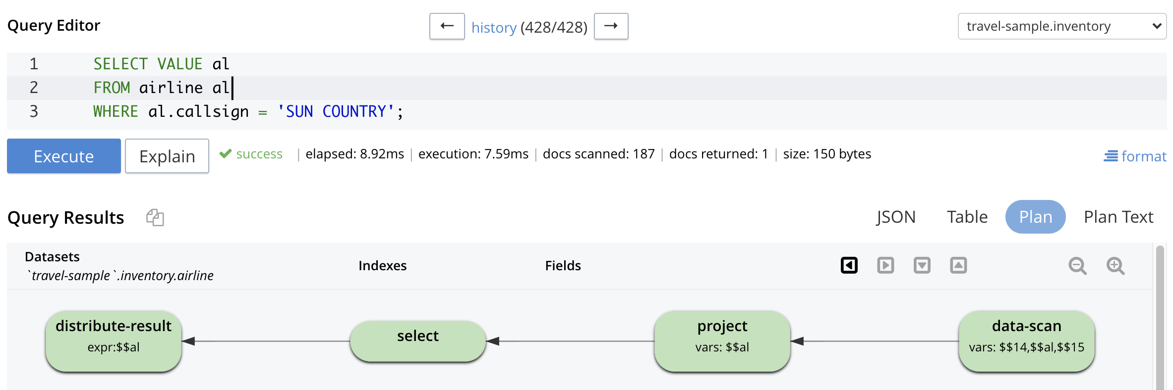
This plan involves a data-scan operation performing a scan of the Analytics collection,
a project operation to eliminate all but the desired information (in this case the whole airline object),
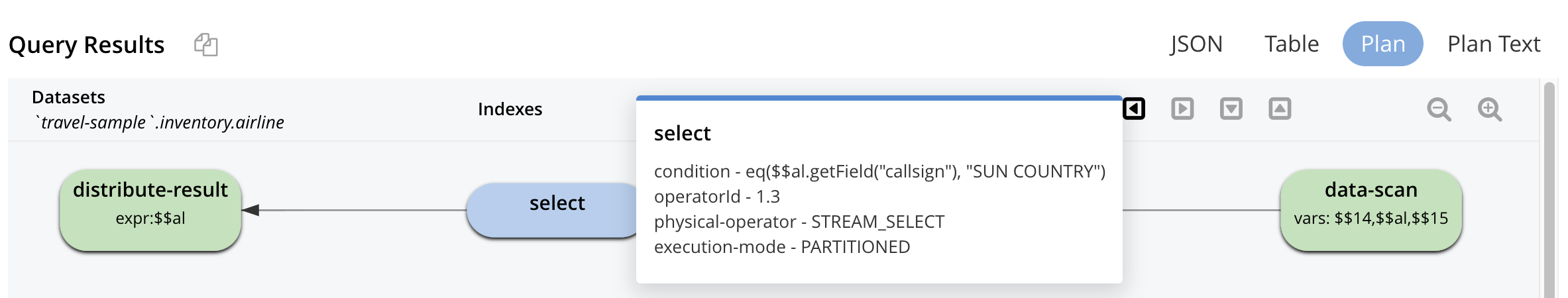
and a select operation to apply the callsign
predicate.
To verify that the select operation is indeed applying the predicate, you can click on it to see more detail:
The following DDL statement can be used to accelerate the execution of this query for a large collection of airlines:
CREATE INDEX callsignidx ON airline (callsign: STRING);Note that a CREATE INDEX statement needs to specify the type as well as the name of the field to be indexed; the
above callsignidx will be used to speed queries that have string-based callsign predicates.
If you execute the query again after creating the index, you will see a more complex query plan that uses the newly created index:
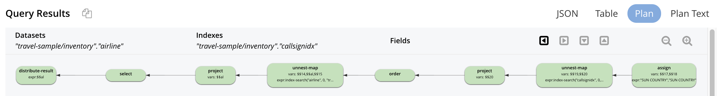
Notice how the plan’s summary line shows that it uses the airline Analytics collection
("travel-sample/inventory"."airline") and its callsignidx secondary index.
The query plan involves first performing an index scan on the secondary index (the first unnest-map operation) to
find airlines whose callsign is "SUN COUNTRY".
Doing so yields a sequence of primary keys for qualifying airlines; that sequence is then sorted (the order
operation) and used to look up the associated airlines (the second unnest-map operation) in the hotel Analytics
collection (using its primary index).
Clicking on a node in the query plan will reveal more of its details.
The remainder of the query plan is similar to the earlier unindexed plan.
Further Help
That’s it! You are now armed and dangerous with respect to semistructured data management using Analytics via SQL++ for Analytics. For more information, see SQL++ for Analytics Reference, or consult the complete list of built-in functions in Builtin Functions.
Couchbase Analytics lets you bring a powerful new NoSQL parallel query engine to bear on your data, using the latest state of the art parallel query processing techniques under the hood. We hope you find it useful in exploring and analyzing your Couchbase Server data — without having to worry about end user performance impact or doing additional schema design and ETL grunt work to make your NoSQL data analyses possible.
Use it wisely, and remember: "With great power comes great responsibility…" 🙂
Do let us know how you like it…!